Special Indexing Techniques: Inverted, Bit map, Cluster, Join indexes

<< Conventional Indexing Techniques: Concept, Goals, Dense Index, Sparse Index

Join Techniques: Nested loop, Sort Merge, Hash based join >>

Lecture-27

Need for Speed: Special Indexing Techniques

Without indexes, th e DBMS may be forced to conduct a full table scan (reading every row in the

table) to locate the desired data, which can be a lengthy and inefficient process. However,

creating indexes requires careful consideration. Although indexes can be quite useful for speeding

data retrieval, they can slow performance of database writes. This slowdown occurs because a

change to an indexed column actually requires two database writes -one to reflect a change in the

table and one to reflect a corresponding change in the index. Thus, if the activities associated with

a table are primarily write -intensive, it is important to make judicious use of indexes on the

relevant tables. Indexes also require a certain amount of disk space, which must be considered

when allocating resources to the database.

Before looking at your indexing options, we must first discuss the two ways to access data: non -

keyed access and keyed access. Non-keyed access uses no index. Each record of the database is

accessed sequentially, beginning with the first record, then second, third and so on. This access is

good when you wish to access a large portion of the database (greater than 85%). Keyed access

provides direct addressing of records. A unique number or character(s) is used to locate and

access records. In this case, when specified records are required (say, record 120, 130, 200 and

500), indexing is much more efficient than reading all the records in between.

Special Index Structures

Inverted index

Bit map index

Cluster index

Join indexes

Table-27.1: Special Index Structures

Inverted index: Concept

An inverted index is an optimized structure that is built primarily for retrieval, with update being

only a secondary consideration. The basic structure inverts the text so that instead of the view

obtained from scanning documents where a document is found and then its terms are seen (think

of a list of documents each pointing to a list of terms it contains), an index is built that maps

terms to documents (pretty much like the index found in the back of a book that maps terms to

page numbers). Instead of listing each document once (and each term repeated for each document

that contains the term), an inverted index lists each term in the collection only once and then

219

shows a list of all the documents that contain the given term. Each document identifier is repeated

for each term that is found in the document.

Within the search engine domain, data are searched far more frequently than they are updated.

This is typical for a data wa rehouse, where updates hardly take place. Given this situation a data

structure called an inverted index commonly used by search engines is also applicable for the data

warehouse environment.

An inverted index is able to do many accesses in O (1) time at the price of significantly longer

time to do an update, in the worst case O(n). Index construction time is longer as well, but query

time is generally faster than with a B-tree i.e. O(log n). Since index construction is an off -line

activity, so it is an appropriate tradeoff i.e. shorter query times at the expense of lengthier index

construction times.

Finally, inverted index storage structures can exceed the storage demands of the document

collection itself. However, the inverted index can be compressed for many systems, to around

10% of the original document collection. Given the alternative (of 26 minute searches), search

engine developers are happy to trade index construction time and storage for query efficiency.

Same is also true for the DSS environment.

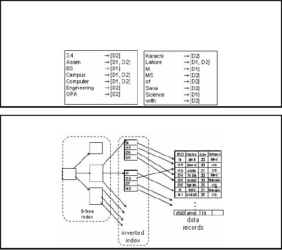
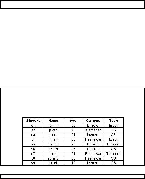
Inverted Index: Example-1

D1: M. Asalm BS Computer Science Lahore Campus

D2: Sana Aslam of Lahore MS Computer Engineering with GPA 3.4 Karachi Campus

Inverted index for the documents D1 and D2 is as follows:

Inverted Index: Example-2

220

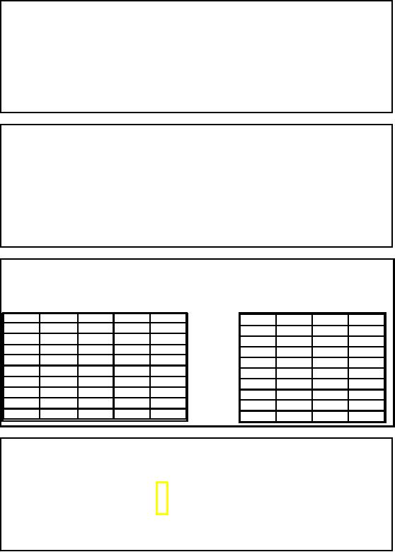
Figure-27.1: Inverted Index: Example-2

Inverted Index: Query

Query:

o Get students with age = 20 and tech = "telecom"

List for age = 20: r4, r18, r34, r35

List for tech = "telecom": r5, r35

Answer is intersection: r35

Bitmap Indexes: Concept

Index on a particular column

Index consists of a number of bit vectors or bitmaps

Each value in the indexed column has a corresponding bit vector (bitmaps)

The length of the bit vector is the number of records in the base table

The ith bit is set to 1 if the ith row of the base table has the value for the indexed column

Bitmap Indexes: Example

The index consists of bitmaps, with a column for each unique value:

Index on City (larger table):

Index on Tech (smaller table):

SID

Islamabad Lahore

Karachi Peshawar

SID

Elect

Telecom

Table-27.2: Bitmap Indexes: Example

Bitmap Index: Query

Query:

§ Get students with age = 20 and campus = "Lahore"

List for age = 20:

1101100000

List for campus = "Lahore": 1010000001

Answer is AND :

1000000000

Good if domain cardinality is small

Bit vectors can be compressed

§ Run length encoding

221

Bitmap Index: Run Length Encoding

Basic Concept

1111000011110000001111100000011111 INPUT

Case-1

14#04#14#06#15#06#15 OUTPUT

1010101010101010101010101010101010 INPUT

Case-2

11#01#11#01#11#01#11#01#... OUTPUT

11111111111111110000000000000000 INPUT

117#017 OUTPUT

Case-3

Bitmap Index: More Queries

Allow the use of efficient bit operations to answer queries, such as:

"Which students from Lahore are enrolled in `CS'?"

Perform a bit -wise AND of two bitmaps: answer s1 and s9

"How many students are enrolled in `CS'?"

Count 1's in the degree bitmap vector

Answer is 4

Bitmaps are not good for high- cardinality textual columns that have numerous values, such as

names or descriptions, because a new column is created in the index for every possible value.

With high -cardinality data and a large number of rows, each bitmap index becomes enormous and

takes a long time to process durin g indexing and retrievals.

Bitmap Index: Adv.

Very low storage space.

Reduction in I/O, just using index.

Counts & Joins

Low level bit operations.

An obvious advantage of this technique is the potential for dramatic reductions in storage

overhead. Consider a table with a million rows and four distinct values with column header of 4

bytes resulting in 4 MB. A bitmap indicating which of these rows are for these values requires

about 500KB.

More importantly, the reduction in the size of index "entries" means that the index can sometimes

be processed with no I/O and, more often, with substantially less I/O than would otherwise be

222

required. In addition, many index-only queries (queries whose responses are derivable through

index scans without searching t he database) can benefit considerably.

Database retrievals using a bitmap index can be more flexible and powerful than a B-tree in that a

bitmap can quickly obtain a count by inspecting only the index, without retrieving the actual data.

Bitmap indexing can also use multiple columns in combination for a given retrieval.

Finally, you can use low-level Boolean logic operations at the bit level to perform predicate

evaluation at increased machine speeds. Of course, the combination of these factors can resu lt in

better query performance.

Bitmap Index: Performance Guidance

Bitmapped indexes can provide very impressive performance speedups; execution times of

certain queries may improve by several orders of magnitude. The queries that benefit the most

from bitmapped indexes have the following characteristics:

The WHERE-clause contains multiple tests on low-cardinality columns

The individual tests on these low-cardinality columns select a large number of rows

The bitmapped indexes have been created on some or all of these low-cardinality

columns

The tables being queried contain many rows

A significant advantage of bitmapped indexes is that multiple bitmapped indexes can be used to

evaluate the conditions on a single table. Thus, bitmapped indexes a e very appropriate for

complex ad-hoc queries that contain lengthy WHERE-clauses. Performance, storage

requirements, and maintainability should be considered when evaluating an indexing scheme.

Bitmap Index: Dis. Adv.

Locking of many rows

Low cardinality

Keyword parsing

Difficult to maintain - need reorganization when relation sizes change (new bitmaps)

Row locking: A potential drawback of bitmaps involves locking. Because a page in a bitmap

contains references to so many rows, changes to a single row inhibit concurrent access for all

other referenced rows in the index on that page.

Low cardinality: Bitmap indexes create tables that contain a cell for each row times each possible

value (the product of the number of rows times the number of unique values). Therefore, a bitmap

is practical only for low- cardinality columns that divide the data into a small number of

categories, such as "M/F", "T/F", or "Y/N" values.

Keyword parsing: Bitmap indexes can parse multiple values in a column into separate keywords.

For example, the title "Marry had a little lamb" could be retrieved by entering the word "Marry"

or "lamb" or a combination. Although this keyword parsing and lookup capability is extremely

223

useful, textual fields tend to contain high -cardinality data (a large number of values) and therefore

are not a good choice for bitmap indexes.

Cluster Index: Concept

A Cluster index defines the sort order on the base table.

Ordering may be strictly enforced (guaranteed) or opportunistically maintained.

At most one cluster index defined per table.

Cluster index may include one or multiple columns.

Reduced I/O.

The big advantage of a cluster index is that all the rows with the same cluster index value will be

placed into adjacent locations in a small number of data blocks.

In this example, all accounts for a specific customer will be clustered into adjacent locations to

increase locality of reference by customer_id.

Cluster indexing allows significant reduction in I/Os when accessing base table via index because

rows with the same index value will be stored into the same blocks. This is a big win for indexed

access for query execution against a single table as well as nested loop joins using indexed

access. Cluster indexing has the effect of transforming a random I/O workload into a sequential

I/O workload when accessing through the cluster index.

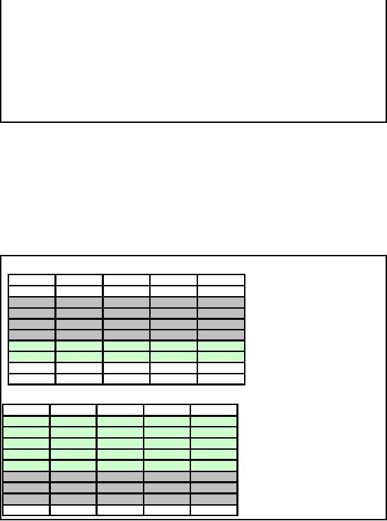
Cluster Index: Example

Student

Name

Age

Campus

Tech

afridi

Lahore

amir

Lahore

Elect

javed

Islamabad

imran

Peshawar

Elect

Cluster indexing on AGE

majid

Karachi

Telecom

salim

Lahore

tahir

Peshawar

Telecom

taslim

Karachi

sohaib

Peshawar

One indexing column at a time

Student

Name

Age

Campus

Tech

afridi

Lahore

javed

Islamabad

salim

Lahore

Cluster indexing on TECH

taslim

Karachi

sohaib

Peshawar

amir

Lahore

Elect

imran

Peshawar

Elect

majid

Karachi

Telecom

tahir

Peshawar

Telecom

Table-27.3: Cluster Index: Example

224

Cluster Index: Issues

Works well when a single index can be used for the majority of table accesses.

Selectivity requirements for making use of a cluster index are much less stringent than for

a non -clustered index.

o Typically by an order of magnitude, depending on row width.

High maintenance cost to keep sorted order or frequent reorganizations to recover

clustering factor.

Optimizer must keep track of clustering factor (which can degrade over time) to

determine optimal execution plan

Significant performance advantage for query execution, but beware of the overhea d of index

maintenance (and reorganization costs!), at best O (n log n).

Query plans will change (or should change) over time where updates are occurring because

degradation of clustering (e.g., adjacency) will take place over time until a reorganization is

performed. Note that this effect assumes that clustering index does not "force" sorted order, but

rather that sorted order is achieved with initial index build and periodic reorganization. It is also

possible to "force" sorted order at a higher cost upon insert and update operations into the data

warehouse.

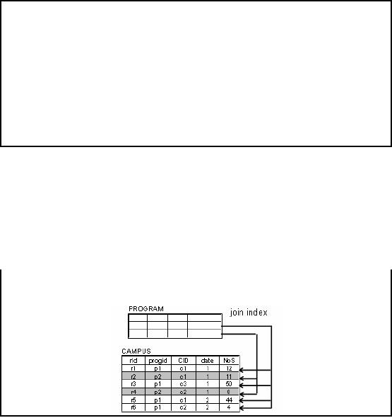
Join Index: Example

The rows of the table consist entirely of such references, which are the RIDs of the relevant rows.

Figure-27.2: Join Index: Example

225

Table of Contents: