Risk and Uncertainty, Measuring risk, Variability of return–Historical Return, Variance of return, Standard Deviation

<< Single period, Multi-period capital rationing, Linear programming

Portfolio and Diversification, Portfolio and Variance, Risk–Systematic & Unsystematic, Beta – Measure of systematic risk, Aggressive & defensive stocks >>

Corporate Finance FIN 622

Lesson 15

RISK AND RETURNS

The following topics will be discussed in this lecture.

Risk and Uncertainty

Measuring risk

Variability of return Historical Return

Variance of return

Standard Deviation

RISK AND UNCERTAINTY:

If you buy an asset or any stock or share, the gains or losses you get on this investment are called return on

investment. This return has normally two components. First, it is the income part that you may receive in

terms of dividend (owning a share) and second part comes from the capital appreciation or increase in the

market value of that share.

The above discussion suggests that the reward of return you get is the due to bearing the risk. Risk refers to

the variability of returns. You may get dividend on a share say 2% or 15%, or even you may not get

anything from the issuing firm. Look at this simple example: the expected returns (income part only) can

vary from 0 to 15%. This is called risk. However, you can use probabilities to determine your return. For

instance, if the economy remains in boom, which has 60% chances, then our return will be 8%. So attaching

probability we can to some extent, determine the return under risk conditions.

The other important thing to remember is that greater the risk, larger the profit.

Uncertainty, refers to a situation where our ability to attach a probability to an outcome is ceased.

From hereafter, we shall discuss the ways and means to measure the risk.

HISTORICAL RETURN ANALYSIS:

The problem with most financial planning is they accept a return rate on each of your investments and

project your financial future on those rates. The argument is over a span of years your investments will

return that rate "on average." Unfortunately this is an invalid and risky assumption. Investment rates vary

from year to year. Sometimes they vary greatly. We cannot accurately predict the return rate on investments

or the inflation rate. Consider the following simple example

You have $1000.00 invested and you expect a 10.0% average yearly return on your investment. In two years

your investment will be worth $1210.00.

Now lets assume your same $1000.00 returns -10.00% the first year and +30.00% the second. Your

investments after those two years are worth only $1170.00 even though your investment returned "on

average" 10.0%.

The above example demonstrates the need for a mechanism to account for the volatility of investment

return rates and the variability of inflation. The J&L Financial Planner has chosen to include two

alternatives, a Monte Carlo Analysis and a Historical Return Analysis, as that mechanism.

J&L Financial Planner's Historical Return Analysis

The following paragraphs outline how the Historical Return Analysis is implemented by the J&L Financial

Planner.

The J&L Financial Planner allows you to create simple or complex financial scenarios (financial plans)

revolving around your existing accounts consisting of investment, retirement, asset, and equity accounts.

The planner allows you to create and assign up to 10 asset allocation classes for each of your accounts. A

simple example would have you create three asset allocation classes Stocks, Bonds, and Cash. You would

assign each account the percentage of each of its allocation classes. A mutual fund account may consist of

70 percent Stocks and 30 percent Bonds, whereas a savings account would be 100 percent Cash. For each

allocation class you assign a historical return data file representing the returns for that class over an

historical time span. The planner comes with 6 example data files including 2 stock files, 2 bond files, 1 cash

file, and an inflation file covering the years 1928 through 2003. The files are provided as examples and

should be replaced with data files which meet your needs. You can create and edit up to 10 files, each

corresponding to an asset allocation class.

The planner gives you two options with the Historical Return Analysis.

The first allows you to execute your financial plan over the historical time span. This generates your net

worth for each year of your plan based on the returns of the historical data starting with the first year of the

Corporate Finance FIN 622

data. In the provided files this would generate a net worth (a line graph) starting with the returns from 1928.

Next it would generate a net worth starting with the returns from 1929. It would do this for each year of

your financial plan.

The second allows you to randomly select return data from the historical data files and use that data to

calculate your net worth over the span of your financial plan. It also gives you the option of selecting the

number of sequential years the program will use. In other words, if you select 10 years of sequential data,

the program randomly selects the first year and then uses the data from the files for the following 9 years

before randomly selecting another year. For example if you choose the number of sequential years as 1 and

select 1000 trials it will randomly select return data from the historical data files for each year of your plan

and execute your plan 1000 times. This has the effect of a Monte Carlo analysis with the random data being

randomly selected from real historical return data.

Summary

In summary, the Historical Return Analysis is able to estimate the probability of achieving the success of

your scenario by accounting for the yearly variability in the two main factors contributing to its outcome,

the return rate on your investments and the inflation rate. You can execute up to a thousand trials of your

scenario. Each trial is a fully independent execution of your financial plan, where each year the return rate

on your investments and the inflation rate can take on a range of values based on historical asset class return

data.

The large number of trials allows the analysis to compute the statistical probability your financial plan will

be successful. For example, if after 1000 trials, 750 of those trials achieved your financial goals, your

financial plan success rate is 75.0%.

If your financial plan success rate is below your expectations the J&L Financial Planner allows you to make

easy scenario changes to play "what-if" with your financial future.

VARIANCE OF RETURN:

The variance essentially measures the average squared difference between the actual returns and the average

return. The bigger this number is, the more the actual returns tend to differ from the average return. Also,

the larger the variance is the ore spread out the returns will be.

It is pertinent to note here that calculating variance and standard deviation will be different for historical

and projected returns.

This is usually very close to the correlation squared. To understand what variance explained means, think of

a manager and a Style Benchmark. Any variance in the difference between manager and Style Benchmark,

i.e., any variance in the excess return of manager over benchmark, represents a failure of the Style

Benchmark variance to explain the manager variance. Hence, the quotient of variance of excess return over

variance of manager represents the unexplained variance. The variance explained is 1 minus the unexplained

variance:

Variance Explained = 1 - Var (e) / Var (M)

Where:

Var (M) = variance of manager returns

Var (e) = variance of excess return of manager over benchmark

STANDARD DEVIATION:

Were this set a sample drawn from a larger population of children, and the question at hand was the

standard deviation of the population, convention would replace the N (or 4) here with N-1 (or 3).

The standard deviation of a probability distribution is defined as the square root of the variance ,

(1)

(2)

Where

is the mean,

is the second raw moment, and denotes an expectation value.

is therefore equal to the second central moment (i.e., moment about the mean),

The variance

(3)

Corporate Finance FIN 622

The square root of the sample variance of a set of

values is the sample standard deviation

(4)

The sample standard deviation distribution is a slightly complicated, though well-studied and well-

understood, function.

However, consistent with widespread inconsistent and ambiguous terminology, the square root of the bias-

corrected variance is sometimes also known as the standard deviation,

(5)

Physical scientists often use the term root-mean square as a synonym for standard deviation when they refer

to the square root of the mean squared deviation of a quantity from a given baseline.

The standard deviation arises naturally in mathematical statistics through its definition in terms of the

second central moment. However, a more natural but much less frequently encountered measure of average

deviation from the mean that is used in descriptive statistics is the so-called mean deviation.

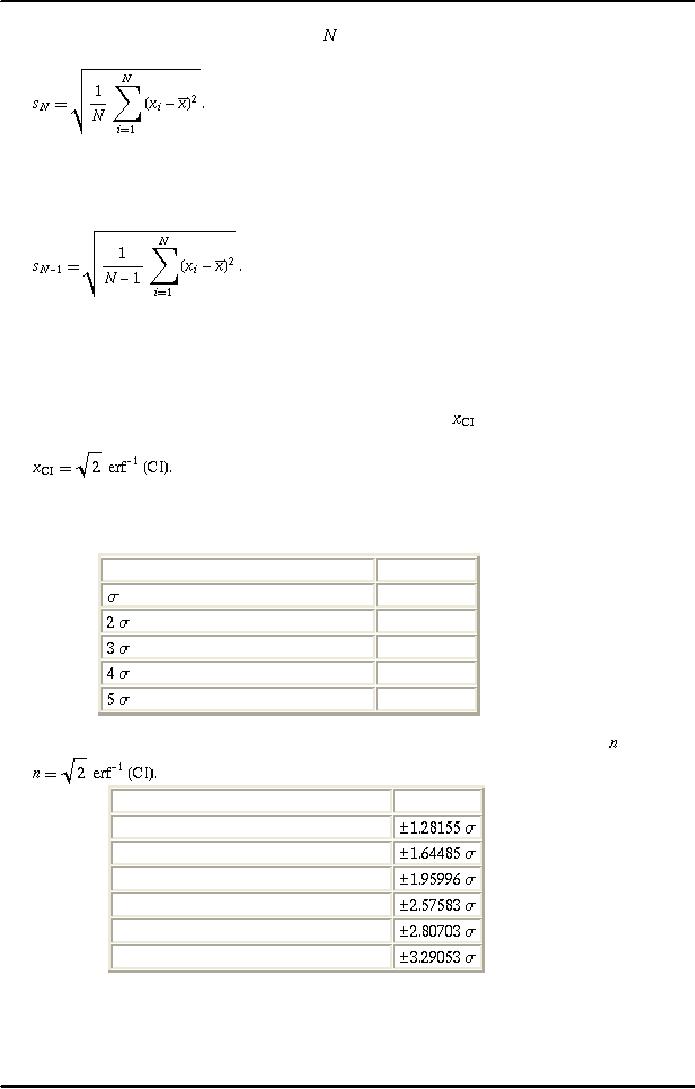
The variants value producing a confidence interval CI is often denoted , and

(6)

The following table lists the confidence intervals corresponding to the first few multiples of the standard

deviation.

Range

0.6826895

0.9544997

0.9973002

0.9999366

0.9999994

To find the standard deviation range corresponding to a given confidence interval, solve (5) for , giving

(7)

range

0.800

0.900

0.950

0.990

0.995

0.999

Table of Contents: