 |
Microeconomics
ECO402
VU
Lesson
21
Production
with Two Outputs--Economies of
Scope
Economies of
scope exist when the
joint output of a single
firm is greater than the
output
that
could be achieved by two
different firms each
producing a single
output.
Examples:
Chicken
farm--poultry and
eggs
Automobile
company--cars and
trucks
University--Teaching
and research
What
are the advantages of joint
production?
Consider an
automobile company producing
cars and tractors
Advantages
1)
Both use capital and
labor.
2)
The firms share management
resources.
3)
Both use the same
labor skills and type of
machinery.
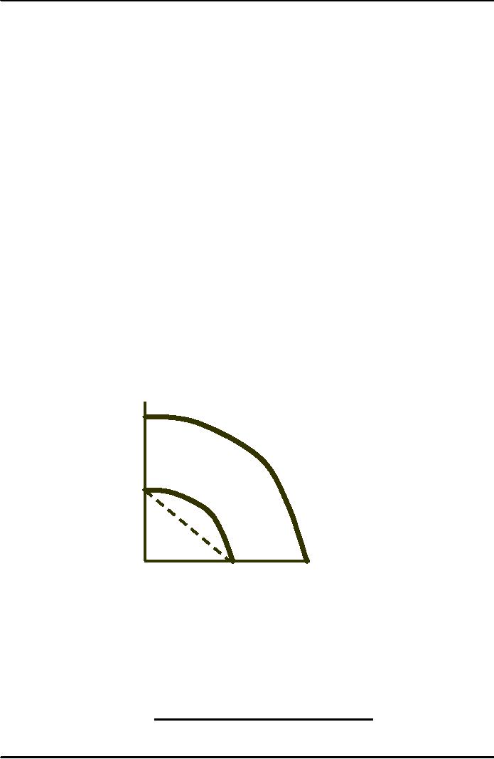
Production:
Firms must
choose how much of each to
produce.
The alternative
quantities can be illustrated
using product transformation
curves.
Product
Transformation Curve
Each
curve shows
Number
combinations
of output
of
tractors
with
a given
combination
of
L &
K.
O1 illustrates a
low
O2
level
of output. O2
illustrates
a higher level
of
output with two
times
as
much labor and
O1
capital.
Number
of cars
Observations
Product
transformation curves are
negatively sloped
Constant
returns exist in this
example
Since the
production transformation curve is
concave is joint production
desirable?
There is no
direct relationship between
economies of scope and
economies of scale.
May experience
economies of scope and
diseconomies of scale
May have
economies of scale and not
have economies of
scope
The
degree
of economies of scope measures
the savings in cost and
can be written:
C(
Q
1 ) +
C
(
Q
2 ) -
C
(
Q
1 , Q
2 )
SC
=
C
(
Q
1, Q
2 )
106
Microeconomics
ECO402
VU
C(Q1) is
the cost of producing Q1
C(Q2) is
the cost of producing Q2
C(Q1Q2)
is the joint cost of
producing both
products
Interpretation:
If SC > 0 -- Economies of
scope
If SC < 0 -- Diseconomies
of scope
Issues
Truckload
versus less than truck
load
Direct versus
indirect routing
Length of
haul
Economies
of Scope in the Trucking
Industry
Questions:
Economies of
Scope
Are
large-scale, direct hauls
cheaper and more profitable
than individual hauls
by
small
trucks?
Are there
cost advantages from
operating both direct and
indirect hauls?
Empirical
Findings
An analysis of
105 trucking firms examined
four distinct
outputs.
Short
hauls with partial
loads
Intermediate
hauls with partial
loads
Long
hauls with partial
loads
Hauls
with total loads
Results
SC = 1.576
for reasonably large
firm
SC = 0.104
for very large
firms
Interpretation
Combining
partial loads at an intermediate
location lowers cost
management
difficulties
with very large
firms.
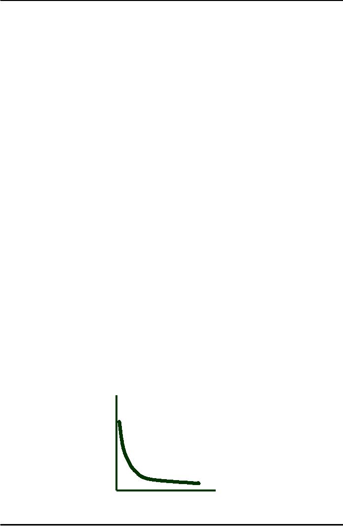
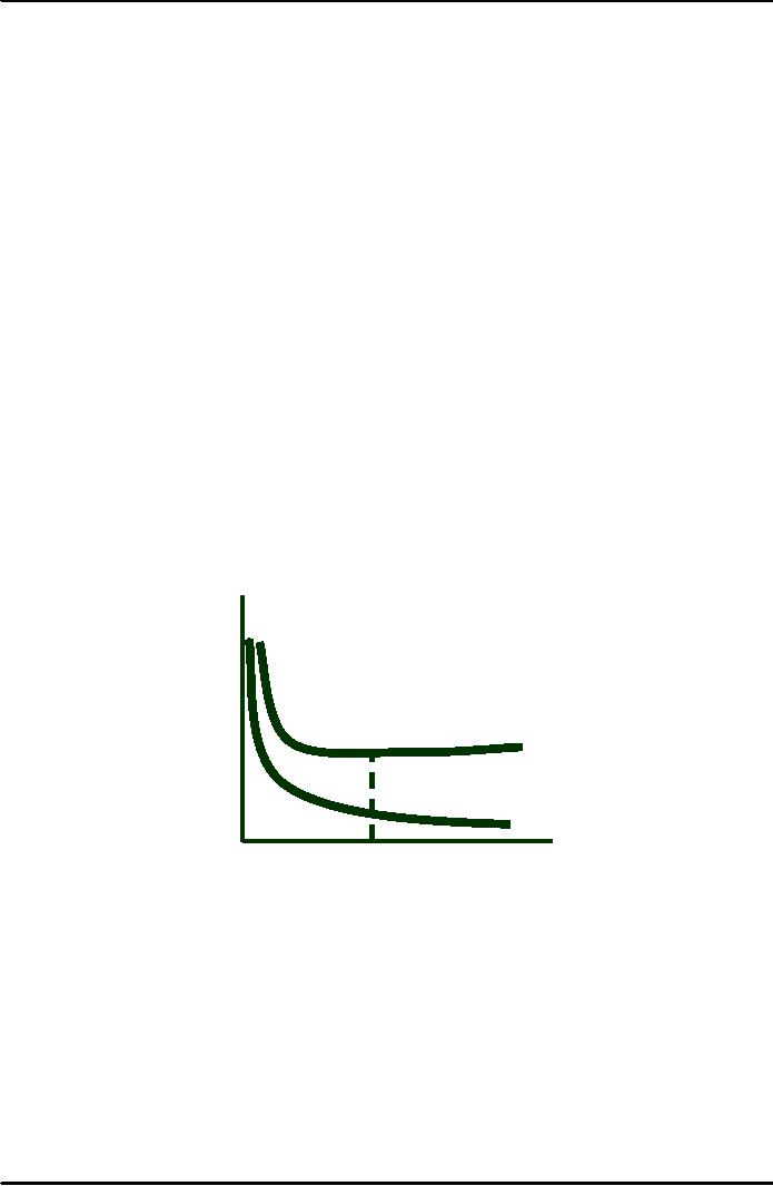
Dynamic
Changes in Costs--The Learning
Curve
The
learning
curve measures
the impact of worker's
experience on the costs
of
production.
It
describes the relationship
between a firm's cumulative
output and amount of
inputs
needed
to produce a unit of
output.
Hours
of labor
per
machine lot
10
8
6
4
2
Cumulative
number of
machine
lots produced
0
20
30
40
50
10
107
Microeconomics
ECO402
VU
The
horizontal axis measures the
cumulative number of hours of
machine tools the firm
has
produced
The
vertical axis measures the
number of hours of labor
needed to produce each
lot.
The
learning curve in the figure
is based on the
relationship:
L
= A + BN-β
If
N=1
L equals A + B
and this measures labor
input to produce the first
unit of output
If
β = 0
Labor input
remains constant as the
cumulative level of output
increases, so there is no
learning
If
β > 0 and N
increases
L approaches A,
and A represent minimum
labor input/unit of output
after all learning
has
taken place.
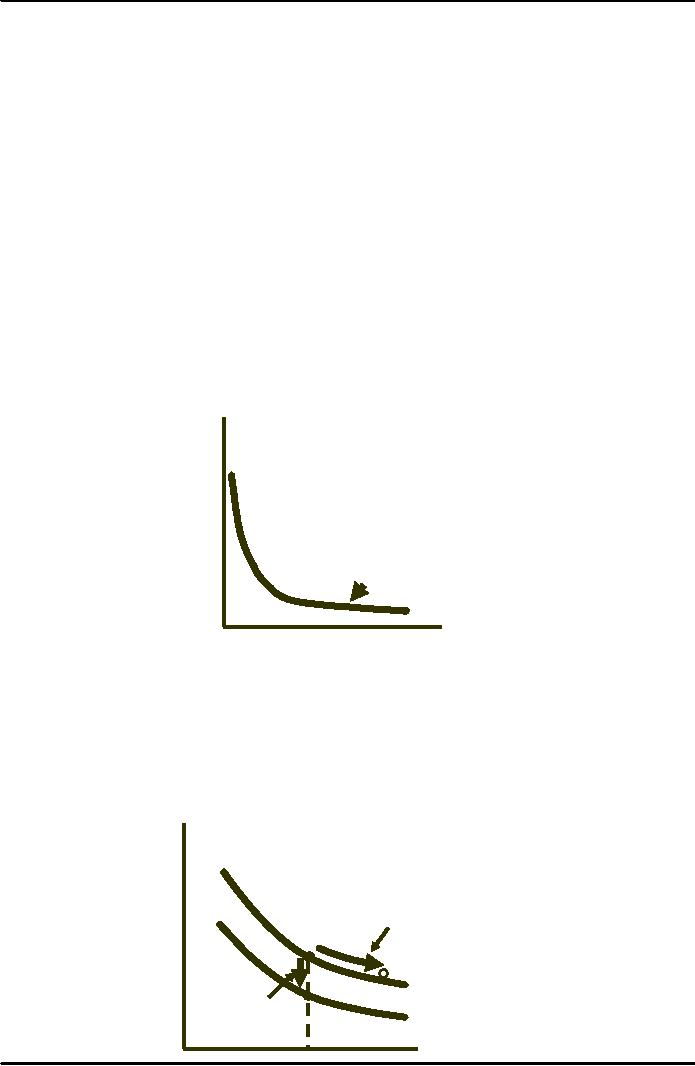
The
larger β:
The more
important the learning
effect.
The
chart shows a sharp
drop
Hours
of labor
in
lots to a cumulative amount
of
per
10
20,
then small savings at
machine
lot
higher
levels.
8
Doubling
cumulative output
causes
a
20% reduction in the
difference
6
between
the input required
and
minimum
attainable input
requirement
4
β
=
0.31
2
Cumulative
number
of
machine lots
0
50
20
30
10
40
produced
Observations
1)
New firms may experience a
learning curve, not
economies of scale.
2)
Older firms have relatively
small gains from
learning.
Economies
of Scale Versus
Learning
Cost
($
per unit
of
output)
Economies
of
Scale
A
B
AC1
Learning
C
AC2
Output
108

Microeconomics
ECO402
VU
Predicting
the Labor Requirements of
Producing a Given
Output
Cumulative
Output
Per-Unit
Labor Requirement
Total
Labor
(N)
for
each 10 units of Output
(L)
Requirement
10
1.00
10.0
20
.80
18.0
(10.0 + 8.0)
30
.70
25.0
(18.0 + 7.0)
40
.64
31.4
(25.0 + 6.4)
50
.60
37.4
(31.4 + 6.0)
60
.56
43.0
(37.4 + 5.6)
70
.53
48.3
(43.0 + 5.3)
80
and over
.51
53.4
(48.3 + 5.1)
The
learning curve
implies:
1)
The labor requirement falls
per unit.
2)
Costs will be high at first
and then will fall
with learning.
3)
After 8 years the labor
requirement will be 0.51 and
per unit cost will be
half
what
it
was in the first year of
production?
Learning
Curve in Practice
Scenario
A new firm
enters the chemical
processing industry.
Do
they:
1)
Produce a low level of
output and sell at a high
price?
2)
Produce
a high level of output and
sell at a low price?
How
would the learning curve
influence your
decision?
The
Empirical Findings
Study of 37
chemical products
Average
cost fell 5.5% per
year
For each
doubling of plant size,
average production costs
fall by 11%
For each
doubling of cumulative output,
the average cost of
production falls by
27%
Which
is more important, the
economies of scale or learning
effects?
Other
Empirical Findings
In the
semi-conductor industry a study of
seven generations of DRAM
semiconductors
from
1974-1992 found learning
rates averaged 20%.
In the
aircraft industry the
learning rates are as high
as 40%.
Applying
Learning Curves
109
Microeconomics
ECO402
VU
1)
To
determine if it is profitable to enter an
industry.
2)
To
determine when profits will
occur based on plant size
and cumulative
output.
Estimating
and Predicting
Cost
Estimates
of future costs can be
obtained from a cost
function, which relates the
cost of
production
to the level of output and
other variables that the
firm can control.
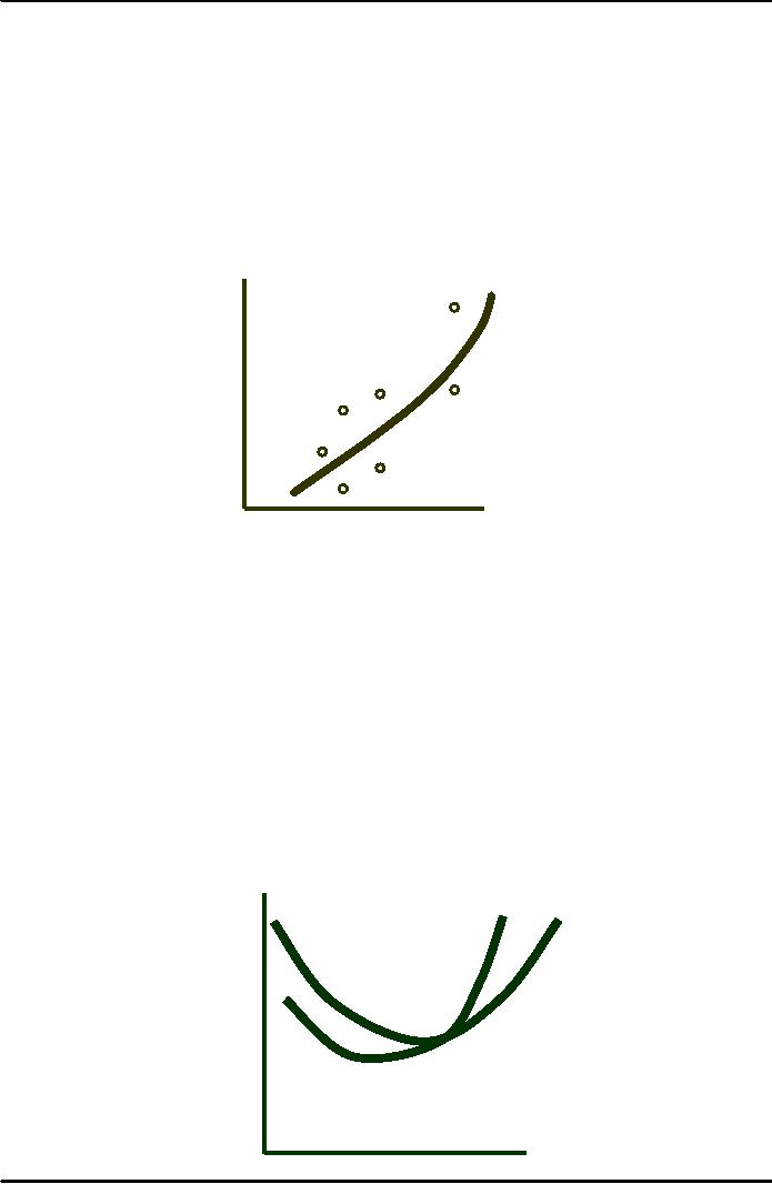
Suppose
we wanted to derive the
total cost curve for
automobile production.
Total
Cost Curve for the
Automobile Industry
Variable
General
Motors
cost
Nissa
Toyot
Hond
Volvo
For
Chrysle
Quantity
of Cars
Estimating
and Predicting
Cost
A
linear cost function (does
not show the U-shaped
characteristics) might
be:
β Q
=
VC
The
linear cost function is
applicable only if marginal
cost is constant.
Marginal cost
is represented by β.
If
we wish to allow for a
U-shaped average cost curve
and a marginal cost that is
not
constant,
we might use the quadratic
cost function:
=
β Q
+ γ Q
2
VC
If
the marginal cost curve is
not linear, we might use a
cubic cost function:
VC
=
β Q
+ γ Q
+δQ
2
3
Cost
($
per unit)
MC
= β + 2γ Q + 3δ Q2
=
β + γQ
+
δQ
2
AVC
Output
(per
time period)
110
Microeconomics
ECO402
VU
Cubic
Cost Function
Difficulties
in Measuring Cost
1)
Output data may represent an
aggregate of different type of
products.
2)
Cost data may not
include opportunity
cost.
3)
Allocating cost to a particular
product may be difficult
when there is more than
one
product
line.
Cost
Functions and the
Measurement of Scale
Economies
Scale Economy
Index (SCI)
·
EC
= 1, SCI = 0:
no economies or diseconomies of
scale
·
EC
> 1, SCI is
negative: diseconomies of
scale
·
EC
< 1, SCI is
positive: economies of
scale
Cost
Functions for Electric
Power
Scale
Economies in the Electric
Power Industry
Output
(million kwh)
43
338
1109
2226
5819
Value
of SCI, 1955
.41
.26
.16
.10
.04
Average
Cost of Production in the
Electric Power
Industry
Average
Cost
(dollar/1000
kwh)
6.5
6.0
1955
A
5.5
5.0
1970
6
24
12
18
30
36
Output
(billions of kwh)
Findings
Decline in
cost
·
Not due to
economies of scale
·
Was caused
by:
Lower input
cost (coal & oil)
Improvements in
technology
A
Cost Function for the
Savings and Loan
Industry
The
empirical estimation of a long-run
cost function can be useful
in the restructuring of
the
savings
and loan industry in the
wake of the savings and
loan collapse in the
1980s.
Data
for 86 savings and loans
for 1975 & 1976 in six
western states
111

Microeconomics
ECO402
VU
Q = total assets
of each S&L
LAC = average
operating expense
Q & TC are
measured in hundreds of millions of
dollars
Average
operating cost are measured
as a percentage of total
assets.
A
quadratic long-run average
cost function was estimated
for 1975:
LAC
=
2.38
- 0.6153Q +
0.0536Q
2
Minimum
long-run average cost
reaches its point of minimum
average total cost when
total
assets
of the savings and loan
reach $574 million.
Average
operating expenses are 0.61%
of total assets.
Almost
all of the savings and
loans in the region being
studied had substantially
less than
$574
million in assets.
Questions
1)
What are the implications of
the analysis for expansion
and mergers?
2)
What are the limitations of
using these results?
112
Table of Contents:
- ECONOMICS:Themes of Microeconomics, Theories and Models
- Economics: Another Perspective, Factors of Production
- REAL VERSUS NOMINAL PRICES:SUPPLY AND DEMAND, The Demand Curve
- Changes in Market Equilibrium:Market for College Education
- Elasticities of supply and demand:The Demand for Gasoline
- Consumer Behavior:Consumer Preferences, Indifference curves
- CONSUMER PREFERENCES:Budget Constraints, Consumer Choice
- Note it is repeated:Consumer Preferences, Revealed Preferences
- MARGINAL UTILITY AND CONSUMER CHOICE:COST-OF-LIVING INDEXES
- Review of Consumer Equilibrium:INDIVIDUAL DEMAND, An Inferior Good
- Income & Substitution Effects:Determining the Market Demand Curve
- The Aggregate Demand For Wheat:NETWORK EXTERNALITIES
- Describing Risk:Unequal Probability Outcomes
- PREFERENCES TOWARD RISK:Risk Premium, Indifference Curve
- PREFERENCES TOWARD RISK:Reducing Risk, The Demand for Risky Assets
- The Technology of Production:Production Function for Food
- Production with Two Variable Inputs:Returns to Scale
- Measuring Cost: Which Costs Matter?:Cost in the Short Run
- A Firms Short-Run Costs ($):The Effect of Effluent Fees on Firms Input Choices
- Cost in the Long Run:Long-Run Cost with Economies & Diseconomies of Scale
- Production with Two Outputs--Economies of Scope:Cubic Cost Function
- Perfectly Competitive Markets:Choosing Output in Short Run
- A Competitive Firm Incurring Losses:Industry Supply in Short Run
- Elasticity of Market Supply:Producer Surplus for a Market
- Elasticity of Market Supply:Long-Run Competitive Equilibrium
- Elasticity of Market Supply:The Industrys Long-Run Supply Curve
- Elasticity of Market Supply:Welfare loss if price is held below market-clearing level
- Price Supports:Supply Restrictions, Import Quotas and Tariffs
- The Sugar Quota:The Impact of a Tax or Subsidy, Subsidy
- Perfect Competition:Total, Marginal, and Average Revenue
- Perfect Competition:Effect of Excise Tax on Monopolist
- Monopoly:Elasticity of Demand and Price Markup, Sources of Monopoly Power
- The Social Costs of Monopoly Power:Price Regulation, Monopsony
- Monopsony Power:Pricing With Market Power, Capturing Consumer Surplus
- Monopsony Power:THE ECONOMICS OF COUPONS AND REBATES
- Airline Fares:Elasticities of Demand for Air Travel, The Two-Part Tariff
- Bundling:Consumption Decisions When Products are Bundled
- Bundling:Mixed Versus Pure Bundling, Effects of Advertising
- MONOPOLISTIC COMPETITION:Monopolistic Competition in the Market for Colas and Coffee
- OLIGOPOLY:Duopoly Example, Price Competition
- Competition Versus Collusion:The Prisoners Dilemma, Implications of the Prisoners
- COMPETITIVE FACTOR MARKETS:Marginal Revenue Product
- Competitive Factor Markets:The Demand for Jet Fuel
- Equilibrium in a Competitive Factor Market:Labor Market Equilibrium
- Factor Markets with Monopoly Power:Monopoly Power of Sellers of Labor