PREFERENCES TOWARD RISK:Reducing Risk, The Demand for Risky Assets

<< PREFERENCES TOWARD RISK:Risk Premium, Indifference Curve

The Technology of Production:Production Function for Food >>

Microeconomics ECO402

Lesson 15

Reducing Risk

Three ways consumers attempt to reduce risk are:

1) Diversification

2) Insurance

3) Obtaining more information

Diversification

Suppose a firm has a choice of selling air conditioners, heaters, or both.

The probability of it being hot or cold is 0.5.

The firm would probably be better off by diversification.

Income from Sales of Appliances

Hot Weather

Cold Weather

Air conditioner sales

$30,000

$12,000

Heater sales

12,000

30,000

* 0.5 probability of hot or cold weather

If the firm sells only heaters or air conditioners their income will be either $12,000 or

$30,000.

Their expected income would be:

1/2($12,000) + 1/2($30,000) = $21,000

If the firm divides their time evenly between appliances their air conditioning and heating

sales would be half their original values.

If it were hot, their expected income would be $15,000 from air conditioners and $6,000

from heaters, or $21,000.

If it were cold, their expected income would be $6,000 from air conditioners and $15,000

from heaters, or $21,000.

With diversification, expected income is $21,000 with no risk

Firms can reduce risk by diversifying among a variety of activities that are not closely

related.

Stock Market

How can diversification reduce the risk of investing in the stock market?

Can diversification eliminate the risk of investing in the stock market?

Insurance

Risk averse are willing to pay to avoid risk.

If the cost of insurance equals the expected loss, risk averse people will buy enough

insurance to recover fully from a potential financial loss.

Microeconomics ECO402

The Decision to Insure

Insurance

Burglary

No Burglary

Expected

Standard

(Pr = .1)

(Pr = .9)

Wealth

Deviation

$40,000

$50,000

$49,000

$9,055

Yes

49,000

While the expected wealth is the same, the expected utility with insurance is greater

because the marginal utility in the event of the loss is greater than if no loss occurs.

Purchases of insurance transfers wealth and increases expected utility.

The Law of Large Numbers

Although single events are random and largely unpredictable, the average outcome of

many similar events can be predicted.

Examples

A single coin toss vs. large number of coins

Whom will have a car wreck vs. the number of wrecks for a large group of drivers

Assume:

10% chance of a $10,000 loss from a home burglary

Expected loss = .10 x $10,000 = $1,000 with a high risk (10% chance of a $10,000 loss)

100 people face the same risk

Then:

$1,000 premium generates a $100,000 fund to cover losses

Actuarial Fairness

· When the insurance premium = expected payout

The Value of Title Insurance When Buying a House

A Scenario:

Price of a house is $200,000

5% chance that the seller does not own the house

Risk neutral buyer would pay:

(. 95 [ 200 , 000 ] + . 05 [ 0 ] = 190 , 000

Risk averse buyer would pay much less

By reducing risk, title insurance increases the value of the house by an amount far greater

than the premium.

Value of Complete Information

The difference between the expected value of a choice with complete information and

the expected value when information is incomplete.

Suppose a store manager must determine how many fall suits to order:

100 suits cost $180/suit

50 suits cost $200/suit

The price of the suits is $300

Suppose a store manager must determine how many fall suits to order:

Unsold suits can be returned for half cost.

The probability of selling each quantity is .50.

Microeconomics ECO402

The Decision to Insure

Expected

Sale of 50

Sale of 100

Profit

1. Buy 50 suits

$5,000

2. Buy 100 suits

1,500

12,000

6,750

With incomplete information:

Risk Neutral: Buy 100 suits

Risk Averse: Buy 50 suits

The expected value with complete information is $8,500.

8,500 = .5(5,000) + .5(12,000)

The expected value with uncertainty (buy 100 suits) is $6,750.

The value of complete information is $1,750, or the difference between the two (the amount

the store owner would be willing to pay for a marketing study).

An Example

Per capita packed milk consumption has fallen over the years

The milk producers engaged in market research to develop new sales strategies to

encourage the consumption of packed milk.

Findings

Packed milk demand is seasonal with the greatest demand in the summer

Ep is negative and small

EI is positive and large

Milk advertising increases sales most in the summer.

Allocating advertising based on this information in Karachi increased sales by Rs. 400,000

and profits by 9%.

The cost of the information was relatively low, while the value was substantial.

The Demand for Risky Assets

Assets

Something that provides a flow of money or services to its owner.

The flow of money or services can be explicit (dividends) or implicit (capital gain).

Capital Gain

An increase in the value of an asset, while a decrease is a capital loss.

Risky & Riskless Assets

Risky Asset

· Provides an uncertain flow of money or services to its owner.

· Examples

Apartment rent, capital gains, corporate bonds, stock prices

Riskless Asset

· Provides a flow of money or services that is known with certainty.

· Examples

Short-term government bonds, short-term certificates of deposit

Microeconomics ECO402

Asset Returns

Return on an Asset

The total monetary flow of an asset as a fraction of its price.

Real Return of an Asset

The simple (or nominal) return less the rate of inflation.

Asset Returns

Monetary Flow

Asset Return =

Purchase Price

Flow

$100/yr.

Asset Return =

= 10%

Bond Price

$1,000

Expected vs. Actual Returns

Expected Return

· Return that an asset should earn on average

Actual Return

· Return that an asset earns

Higher returns are associated with greater risk.

The risk-averse investor must balance risk relative to return

Risk and Budget Line

Expected return, RP, increases as risk increases.

The slope is the price of risk or the risk-return trade-off.

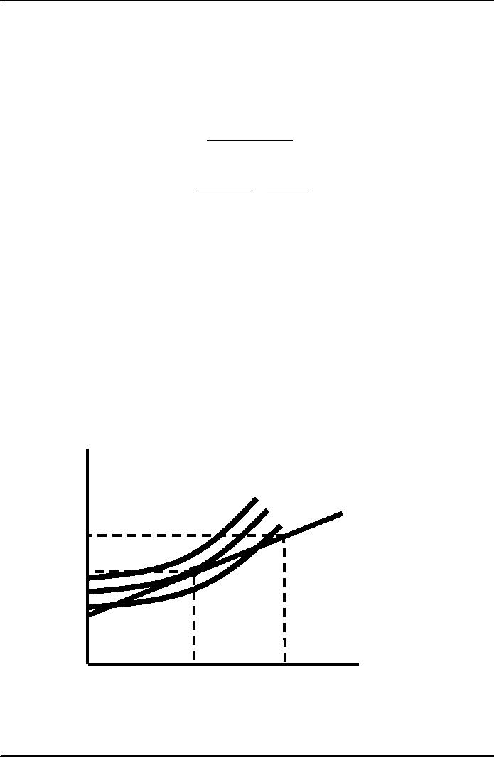
Choosing Between Risk and Return

U2 is the optimal choice of those

obtainable, since it gives the highest return

Expected

for a given risk and is tangent to the budget

Return, Rp

line.

Budget Line

σm

σ∗

σ*

Standard Deviation of

Return, σp

Microeconomics ECO402

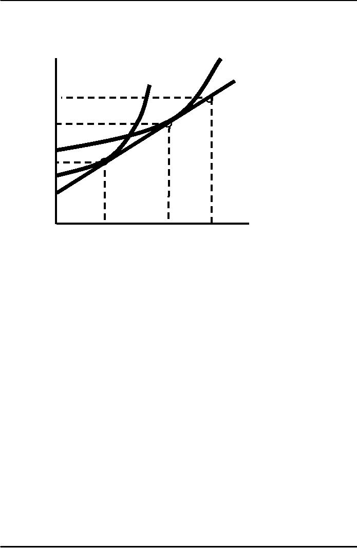
The Choices of Two Different Investors

Expected

Return,Rp

Budget line

Given the same budget

line, investor A chooses

low return-low risk,

while investor B

chooses high return-

high risk.

Standard Deviation

σA

σB

σm

of Return σP

Table of Contents: