 |
PERT / CPM:ALGORITHM FOR CRITICAL PATH, Free Slack |
| << PERT / CPM:DUMMY ACTIVITIES, TO FIND THE CRITICAL PATH |
| PERT / CPM:Expected length of a critical path, Expected time and Critical path >> |
Operations
Research (MTH601)
34
Start
B,6
E,6
Fig.
13
We
see that there are
three paths or routes from
start to end.
The
following are the
paths.
(1)
Start - A - D - End
(2)
Start - B - C - D - End
(3)
Start - B - E - End.
The
times taken to complete the
activities on the three paths
are
5+3
=
8 days
6
+ 7 + 3 = 16 days
6+6
=
12 days
The
longest path is B-C-D and
the duration is 16 days.
Hence the critical path is
B-C-D and the
project
completion
time is 16 days.
Thus,
whether we use the arrow
diagram or the activity on
node diagram, we get the
same result. This
procedure
can be applied without much
effort for small projects involving
only a few activities but
the same
procedure
may be cumbersome if the
project involves a large number of
activities. However, there is an
effective
method
of finding the critical path
as explained in the next
section.
ALGORITHM
FOR CRITICAL PATH
Consider
the following
project.
Job's
name
Immediate
predecessor
Time
to complete the job
a
-
10
days
b
-
3
days
c
a,b
4
days
d
a
7
days
e
d
4
days
f
c,e
12
days
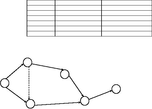
We
draw the project graph by an arrow
diagram as shown in Fig 14.
The activity `g' is a dummy
activity
consuming
no time.
2
d
a
7
10
g 0
4
34
Operations
Research (MTH601)
35
1
4
e
b
6
3
f
c
12
3
5
4
Fig.
14
Early
start and early finish
programme
We
define the 'early start' of
a job in a project as the earliest
possible time when the
job can begin. This
is
the
first number in the bracket.
The early finish time of a
job is its early start time
plus the time required to
perform
the
job. We put this as the second
number in the same bracket.
Thus if in fig. 15 the early
start of the job a will be
0
as
this is the first job. The
early finish 0 + 10 = 10.
For convenience we denote
the start time of a project
as 0. So we
have
early start and early
finish times as (0, 10)
for job a. For job b,
the early start time
will also start and
the early
finish
times are (0, 3).
The jobs d and g can
start, at the earliest, as
soon as the job a is
completed, because 'a' is
the
predecessor
for d and g. Hence the
early start time for
job d will be 10 and early
finish time for job d
will be
10
+ 7 = 17. For the job g
the early start and
early finish will (10,
10) since g happened to be a
dummy job. Next we
take
the job c which has
two predecessors namely b
and g. The job c can be
started, at the earliest on
10. So the job c
can
start, at the earliest only
on 10 and the early finish
of the job c will be 10 + 4 = 14.
Similarly the early start
of
job
e is 17 and finish is 17 + 4 = 21.
The job f has two
predecessors namely c and e, c is
finished at the earliest on 14
and
e on 21. So, the job f can
start at the earliest only
on 21 and finished at the earliest on
33.
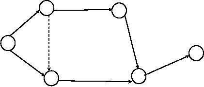
All
the above data are
recorded as shown in figure
15.
d(10,17)
2
4
(0,10)
7
a
g
10
(10,10)
4 e
1
(17,21)
b
6
(0,3)
(21,33)
3
f
3
c
(10,14)
5
12
4
Early
- Start
Early
- Finish
Schedule
Fig.
15
35
Operations
Research (MTH601)
36
Thus
the project can be completed
in 33 days. If the earliest completion
time of the project is 33
days
after
it has begun, the longest
path through the network
must be 33 days in length.
When we compare the
alternate
paths
available for completion of the
project (a-d-e-f = 33;
a-g-c-f = 26; b-c-f = 19)
from the beginning to the
end we
will
find that the critical
path is 33 days, with the
jobs a, d, e, f on the critical
path.
Late
start and Late finish
programme
The
activities not on the critical
path can be delayed without
delaying the completion date of
the project. A
normal
question may arise at this
juncture as to how much
delay can be allowed for non-critical
jobs. How late can
a
particular
activity be started and
still maintain the length of
the project duration? For
answering these questions
we
find
the late start and
late finish times for
each activity in the project
graph.
We
define the late start of an
activity as the latest time
that it can begin without
pushing the finish date
of
the
project further into the
future. Similarly late
finish of an activity is the
late start time plus
the activity
duration.
We
have seen that the
early start and early
finish time of activities are
calculated in the forward
direction
from
left to right. To calculate the
late start and late
finish times, we begin at
the end of the network and
work
backwards.
In the example cited above
we begin with the node 6.
The job leading to the
node is job f. It must be
completed
by day 33 so as not to delay
the project. Therefore, day
33 is the latest finish. In
general duration of
the
critical
path will be taken as the
late finish time of the
project.
The
time taken for the
activity f is 12 days, so that it
must begin at day 21 and
end on 33. Thus the
late start
of
the activity f is day
21.
We
represent the late start
and late finish times of
the activity f within
brackets (21, 33) in
figure16. The
job
f has two predecessors
namely c and e. The late-finish
times for both jobs
can be take as day 21. If
this is so, c's
late
start will be 21-4 or day 17
and e's late start
will be 21-4 or day 17. We
can record the late
start and late
finish
times
jobs c and e in the figure
within brackets.
Now,
the job d is the only
predecessor to e and d can
finish as late as day 17
which is the late start of
e, so d
can
start as late as on day 10.
Coming to the activity g, which is
the predecessor to c, the
late finish time of job g
is
the
same as late start time of
c. So late start and late
finish time of g will be
(17, 17). Since b precedes
c, b also can
finish
as late as on day 17 and
start as late as on day
14.
a
2
d
(10, 17)
(0,
10)
1
4
e
g
(17, 17)
(17,
21)
b
(21,
33)
6
(14,
17)
3
f
c
(17,
21)
5
Late
- Start
Late
- Finish
Schedule
36
Operations
Research (MTH601)
37
Fig.
16
Next
we take job a, which has
two successors namely d and
g, which have days 10 and 17
as the late start
times
respectively. So the job a must
finish as late as on day 10 in
order that a can be made to
start on day 10.
The
finish
time of the activity a will
be least of the late start
time of the successor activities.
Hence the late finish of
the
activity
a must be day 10 and it
starts on day 0. This is also
shown figure 16.
The
above information of early start-early
finish programme and late
start-late finish programmes is
very
useful
as we shall see next.
Slack
or Float
In
the figure 15 and figure 16 which
represent the early
start-early finish and late
start-late finish
programmes,
we observe that the late
start and early start
times are identical for some
jobs. (Similarly late and
early
finish
times). For example for
the job a, the early
and late start time is 0,
for the job d, early
and late start time is
10,
for
e they are 17 and for f
also they are 21,
whereas for job b the
early start is day 0 and
late start is day 14.
This
indicates
that the job b can start as
early as day 0 or as late as on
day 14, without delaying
the project completion
date
of 33 days. This difference between
late start of the job and
the early start of the
same job is called as
'slack' or
'float'.
It is also termed as 'total
slack' or 'total float'. This denotes
the maximum delay that
can be allowed for this
job.
Similarly for job g, the
early start time is day 10
and late start time is
17. There is a difference of 7
days which
is
the slack for job 'g'.
Similarly we have a slack of 7
days for the job 'c'
also.
The
jobs having no slack thus
become critical and the
jobs with slacks are
non-critical. So if we connect the
jobs
having no slacks, we get the
critical path. This is the
method of finding the
critical path. In the
example the jobs
a,
d, e, f have no slack and
the path connecting a, d, e
and f or 1-2-4-5-6 becomes
the critical path.
We
can summaries the slack
for all jobs given in
the tabular below.
Jobs
Early
Early
Late
Late
Slack
start
finish
start
finish
a
0
10
0
10
0
b
0
3
14
17
14
c
10
14
17
21
0
d
10
17
10
17
0
e
17
21
17
21
0
f
21
33
21
33
0
g
10
10
17
17
7
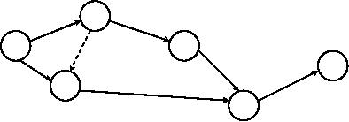
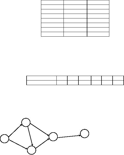
This
critical path is shown in figure
17
a
d
g
37
Operations
Research (MTH601)
38
b
e
c
f
Fig.
17
Free
Slack:
Free
Slack is defined as the
amount of time an activity
can be delayed without affecting
the early start
time
of
any other job. In other
words, the free slack of
any activity is the
difference between its early
finish time and
the
earliest
of the early start times of
all its immediate successors. In the
example above, if we take
the activity b, its
early
finish time is day 3 and its
immediate successor c starts at the
earliest on day 10. 'c'
can start as late as on
day
17,
but there is not compulsion
on c to start exactly on day 10. If he
chooses to start on day 10
(earliest start time)
ten
b will b\have only 7 days as
free slack (difference
between early start of c and
early finish of b).
Similarly for the
job
c also we have free slack as
the difference between the
early finish of c and early
start of its immediate successor
'f'
i.e. 21-14 = 7 days. Free
slack can never exceed total
slack. The total slack and
free slack for all
activities are
given
in the following
table.
Activity
Total
Slack
Free
Slack
a
0
0
b
14
7
g
7
0
c
0
7
d
0
0
e
0
0
f
7
0
Independent
slack:
It
is that portion of the total
float within which an
activity can be delayed for
start without affecting
slacks
of
the preceding activities. It is computed
by subtracting the tail
event slack from the
free float. If the result
is
negative
it is taken as zero.
Example
The
following table gives the
activities of a construction project and
duration.
Activity
1-2
1-3
2-3
2-4
3-4
4-5
Duration
(days)
20
25
10
12
6
10
(i)
Draw the network for the
project.
(ii)
Find the critical
path.
(iii)
Find the total, free
and independent floats each
activity.
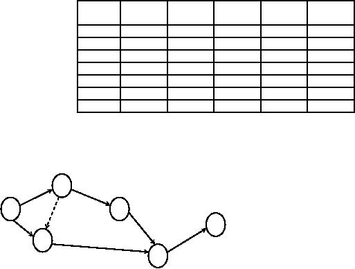
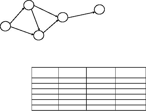
Solution:
The
first step is to draw the network
and fix early start
and early finish schedule
and then late
start-late
finish schedule as in figure 18 and
figure 19.
38
Operations
Research (MTH601)
39
2
(20,
32)
(0,
20)
20
12
10
(20, 30)
4
10
5
1
25
(36,
46)
6
(30,
36)
(0,
25)
3
Early-Start
Early-Finish
Schedule
Fig.
18
(24,
36)
2
5
(0,
20)
(20,
30)
4
(36,
46)
1
(30,
36)
(5,
30)
3
Late-Start
Late-Finish
Schedule
Fig.
19
Activity
Total
Slack
Free
Slack
Independent
Slack
1-2
0
0
0
1-3
5
5
5
2-3
0
0
0
2-4
4
4
4
3-4
0
0
0
4-5
0
0
0
To
find the critical path,
connect activities with 0 total
slack and we get 1-2-3-4-5
as the critical path.
Check
with alternate paths.
1-2-4-5
=
42
1-2-3-4-5
= 46*
(critical
path)
1-3-4-5
=
41
5PERT
MODEL
39

Operations
Research (MTH601)
40
PERT
was developed for the
purpose of solving problems in aerospace
industries, particularly in
research
and
development programmes. These
programmes are subject to
frequent changes and as such
the time taken to
complete
various activities are not
certain, and they are
changing and non-standard.
This element of uncertainty
is
being
specifically taken into account by
PERT. It assumes that the
activities and their network
configuration have
been
well defined, but it allows
for uncertainties in activity
times. Thus the activity
time becomes a random
variable.
If
we ask an engineer, or a foreman or a
worker to give a time estimate to
complete a particular task, he
will at once
give
the most probable time
required to perform the
activity. This time is the
most likely time estimate
denoted by
tm. It is
defined as the best possible
time estimate that a given
activity would take under
normal conditions
which
often
exist.
But
he is also asked to give two
other time estimates. One of
these is a pessimistic time
estimate. This is the
best
guess of the maximum time
that would be required to perform an
activity under the most
adverse circumstances
like
(1)
supply
of materials not in
time
(2)
non-cooperation
from the workers
(3)
the
transportation arrangements not
being effective etc.
Thus
the pessimistic time
estimate is the longest time
the activity would require
and is denoted by tp.
On
the
other hand if everything
goes on exceptionally well or under
the best possible
conditions, the time taken
to
complete
an activity may be less than
the most likely time
estimate. This time estimate is
the smallest time
estimate
known
as the optimistic time
estimate and denoted by
to.
Thus,
given the three time
estimates for an activity, we
have to find the expected
duration of an activity or
expected
time of an activity as a weighted
average of the three time
estimates. PERT makes the
assumption that the
optimistic
and pessimistic activity
(to and
tp) are occur. It also
assumes that the most
probable activity time tm,
is four
times
more likely to occur than
either of the other two.
This is based on the
properties of Beta distribution.
Beta
distribution
was chosen as a reasonable approximation
of the distribution of activity times.
The Beta distribution is
unimodel,
has finite non-negative end
points and is not
necessarily symmetrical-all of which seen
desirable
properties
for the distribution of activity
times. The choice of Beta
distribution was not based on empirical
data.
Since
most activities in a development project
occur just once, frequency distribution
of such activity times
cannot
be
developed from past
data.
So,
if we follow Beta distribution with
weights of 1, 4, 1 for optimistic, mostly
likely and pessimistic
time
estimates
respectively a formula for the
expected time denoted by
te can
be written as
to + 4tm +
t
p
te =
6
For
example if we have 2, 5 and 14
hours as the optimistic
(to),
most likely (tm) and
pessimistic (tp)
time
estimate
then the expected time
for the activity would
be
2+4(5)+14
te =
6
36
=
=
6
hrs
6
40

Operations
Research (MTH601)
41
If
the time required by an
activity is highly variable
(i.e) if the range of our
time estimates is very
large,
then
we are less confident of the
average value. We calculate
them if the range were
narrower. Therefore it is
necessary
to have a means to measure
the variability of the
duration of an activity. One
measure of variability of
possible
activity times is given by
the standard deviation of
their probability distribution.
PERT
simplifies the calculation of
standard deviation denoted by
St as
estimated by the formula,
t
p -
to
St =
6
St is
one sixth of the difference
between the two extreme
time estimates, namely
pessimistic and optimistic
time
estimates.
The variance Vt of
expected time is calculated as
the square of the
deviation.
2
⎛
t
p -
to ⎞
Vt = ⎜
⎜ 6 ⎟
(i.e.)
⎟
⎝
⎠
In
the example above
14-2
St =
=
2
hrs
6
(14-2)2
=
4
hr2
Vt =
2
6
41
Table of Contents:
- Introduction:OR APPROACH TO PROBLEM SOLVING, Observation
- Introduction:Model Solution, Implementation of Results
- Introduction:USES OF OPERATIONS RESEARCH, Marketing, Personnel
- PERT / CPM:CONCEPT OF NETWORK, RULES FOR CONSTRUCTION OF NETWORK
- PERT / CPM:DUMMY ACTIVITIES, TO FIND THE CRITICAL PATH
- PERT / CPM:ALGORITHM FOR CRITICAL PATH, Free Slack
- PERT / CPM:Expected length of a critical path, Expected time and Critical path
- PERT / CPM:Expected time and Critical path
- PERT / CPM:RESOURCE SCHEDULING IN NETWORK
- PERT / CPM:Exercises
- Inventory Control:INVENTORY COSTS, INVENTORY MODELS (E.O.Q. MODELS)
- Inventory Control:Purchasing model with shortages
- Inventory Control:Manufacturing model with no shortages
- Inventory Control:Manufacturing model with shortages
- Inventory Control:ORDER QUANTITY WITH PRICE-BREAK
- Inventory Control:SOME DEFINITIONS, Computation of Safety Stock
- Linear Programming:Formulation of the Linear Programming Problem
- Linear Programming:Formulation of the Linear Programming Problem, Decision Variables
- Linear Programming:Model Constraints, Ingredients Mixing
- Linear Programming:VITAMIN CONTRIBUTION, Decision Variables
- Linear Programming:LINEAR PROGRAMMING PROBLEM
- Linear Programming:LIMITATIONS OF LINEAR PROGRAMMING
- Linear Programming:SOLUTION TO LINEAR PROGRAMMING PROBLEMS
- Linear Programming:SIMPLEX METHOD, Simplex Procedure
- Linear Programming:PRESENTATION IN TABULAR FORM - (SIMPLEX TABLE)
- Linear Programming:ARTIFICIAL VARIABLE TECHNIQUE
- Linear Programming:The Two Phase Method, First Iteration
- Linear Programming:VARIANTS OF THE SIMPLEX METHOD
- Linear Programming:Tie for the Leaving Basic Variable (Degeneracy)
- Linear Programming:Multiple or Alternative optimal Solutions
- Transportation Problems:TRANSPORTATION MODEL, Distribution centers
- Transportation Problems:FINDING AN INITIAL BASIC FEASIBLE SOLUTION
- Transportation Problems:MOVING TOWARDS OPTIMALITY
- Transportation Problems:DEGENERACY, Destination
- Transportation Problems:REVIEW QUESTIONS
- Assignment Problems:MATHEMATICAL FORMULATION OF THE PROBLEM
- Assignment Problems:SOLUTION OF AN ASSIGNMENT PROBLEM
- Queuing Theory:DEFINITION OF TERMS IN QUEUEING MODEL
- Queuing Theory:SINGLE-CHANNEL INFINITE-POPULATION MODEL
- Replacement Models:REPLACEMENT OF ITEMS WITH GRADUAL DETERIORATION
- Replacement Models:ITEMS DETERIORATING WITH TIME VALUE OF MONEY
- Dynamic Programming:FEATURES CHARECTERIZING DYNAMIC PROGRAMMING PROBLEMS
- Dynamic Programming:Analysis of the Result, One Stage Problem
- Miscellaneous:SEQUENCING, PROCESSING n JOBS THROUGH TWO MACHINES
- Miscellaneous:METHODS OF INTEGER PROGRAMMING SOLUTION