Note it is repeated:Consumer Preferences, Revealed Preferences

<< CONSUMER PREFERENCES:Budget Constraints, Consumer Choice

MARGINAL UTILITY AND CONSUMER CHOICE:COST-OF-LIVING INDEXES >>

Microeconomics ECO402

LESSON 8

Note it is repeated

Consumer Preferences

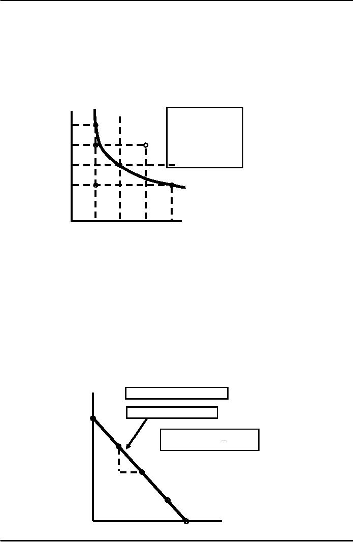
Indifference curves represent all combinations of market baskets that provide the

same level of satisfaction to a person.

Consumer Preferences

Clothing

Combination B,A, & D

(units per week)

yield the same

satisfaction

·E is preferred to U

·U is preferred to H &

Food

(units per week)

Budget Constraints

The Budget Line

The budget line indicates all combinations of two commodities for which total

money spent equals total income.

The Budget Line

Let F equal the amount of food purchased, and C is the amount of clothing.

Price of food = Pf and price of clothing = Pc

Then Pf F is the amount of money spent on food, and PcC is the amount of

money spent on clothing.

The budget line then can be written:

PFF + PCC = I

Clothing

Pc = $2

Pf = $1

I = $80

(units

per week)

Budget Line F + 2C = $80

(I/PC) = 40

Slope = ΔC/ΔF = -

= - PF/PC

Food

(units per week)

80 = (I/PF)

Microeconomics ECO402

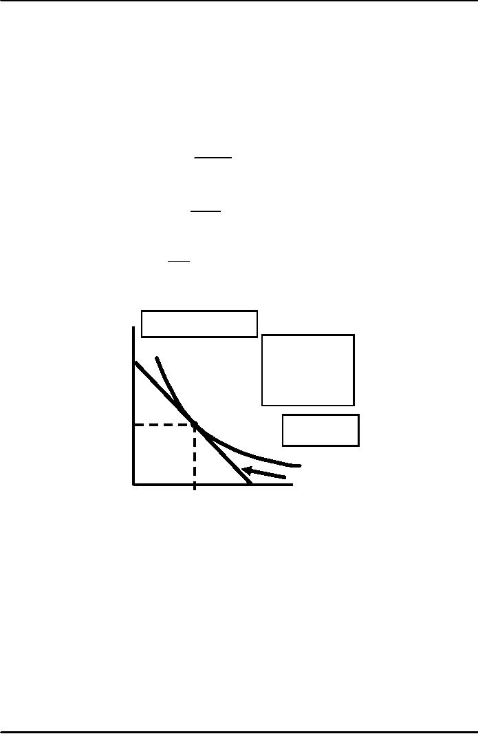
Consumer Choice

Consumers choose a combination of goods that will maximize the satisfaction they can

achieve, given the limited budget available to them.

The maximizing market basket must satisfy two conditions:

It must be located on the budget line.

Must give the consumer the most preferred combination of goods and

services.

Recall, the slope of an indifference curve is:

Δ C

MRS

Δ F

Further, the slope of the budget line is:

= -

Slope

Therefore, it can be said that satisfaction is maximized where:

P F

MRS

P C

Pc = $2

Pf = $1

Clothing

$80

(units per

week)

At market basket A

the budget line and

the

indifference curve are

tangent and no higher

level of satisfaction

can be attained.

At A:

MRS =Pf/Pc =

Budget Line

Food (units per week)

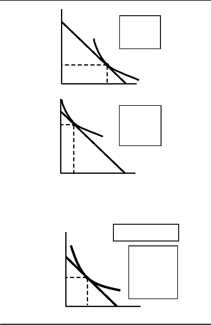
Designing New Automobiles (II)

Consider two groups of consumers, each wishing to spend $10,000 on the

styling and performance of cars.

Each group has different preferences.

By finding the point of tangency between a group's indifference curve and the

budget constraint auto companies can design a production and marketing plan.

Microeconomics ECO402

Styling

These consumers

$10,000

are willing to trade

off a considerable

amount of styling

for some additional

performance

$3,000

$10,000 Performance

$7,000

Styling

These consumers

$10,000

are willing to trade

off a considerable

amount of

$7,000

performance for

some additional

styling

$10,000 Performance

$3,00

Consumer Choice

Decision making & Public Policy

Choosing between a non-matching and matching grant to fund police

expenditures

Non-matching Grant

Private

Expenditures

($)

Before Grant

· Budget line: PQ

·A: Preference maximizing

market basket

·Expenditure

·OR: Private

·OS: Police

Police

Expenditures ($)

Microeconomics ECO402

Non-matching Grant

Private

Expenditures

($)

After Grant

· Budget line: TV

·B: Preference maximizing

market basket

·Expenditure

·OU: Private

·OZ: Police

Police

Expenditures ($)

Private

Before Grant

Expenditures ($)

· Budget line: PQ

Matching Grant

· A: Preference maximizing

market basket

After Grant

·C: Preference maximizing

market basket

Expenditures

·OW: Private

·OX: Police

Police ($)

Private

Expenditures ($)

Matching Grant

Non-matching Grant

·Point B

·OU: Private expenditure

·OZ: Police expenditure

Matching Grant

·Point C

·OW: Private expenditure

·OX: Police expenditure

Z X

Police ($)

Microeconomics ECO402

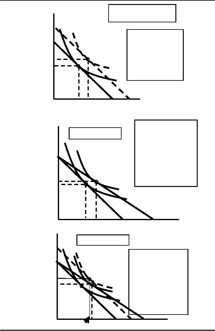
Revealed Preferences

If we know the choices a consumer has made, we can determine what her preferences

are if we have information about a sufficient number of choices that are made when

prices and incomes vary.

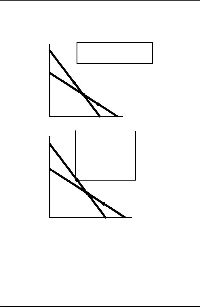
Revealed Preferences--Two Budget Lines

I1: Chose A over B

Clothing

A is revealed preferred to B

(units per

l2: Choose B over D

month)

B is revealed preferred to D

Food (units per month)

Clothing

(units per

All market baskets

month)

in the blue

shaded area are

preferred to A.

B is preferred to

all market baskets

in the pink area

Food (units per month)

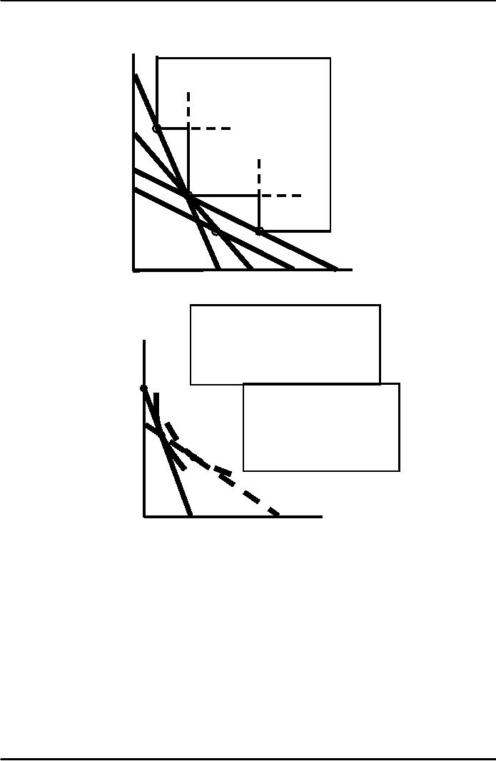
Revealed Preferences--Four Budget Lines

Microeconomics ECO402

I3: E revealed preferred to A

Clothing

(units per

month)

All market baskets in the

blue area preferred to A

A: preferred to all

I4: G revealed preferred to A

market baskets in

the pink area

Food (units per month)

Scenario

·Roberta's recreation budget = $100/wk

Other

Recreational

·Price of exercise = $4/hr/week

Activities

·Exercises 10 hrs/wk at A given U & I

($)

100 C

·The rate changes to $1/hr +

$30/wk

·New budget line I

combination B

·Reveal preference of B to A

Would the Club's

profits increase?

Amount of Exercise

(hours)

Table of Contents: