 |
Operations
Research (MTH601)
148
2
0
1
0
0
1
20
20
S2
First
Iteration: x enters
and S1 leaves the
basis.
RHS
Ratio
Eqn.
Basic
Coefficient
of
No.
Variable
S2
Z
x
y
S1
0
-
1
0
-2
3
0
30
1
0
1
-1
1
0
10
-10
x
2
0
0
1
-1
1
10
10
S2
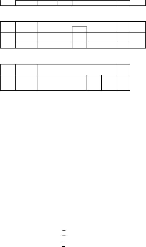
Second
Iteration: y enters
and S2 leaves the
basis.
RHS
Eqn.
Basic
Coefficient
of
No.
Variable
S2
Z
x
y
S1
0
-
1
0
0
1
2
50
1
0
1
0
0
1
20
x
2
0
0
1
-1
1
10
y
From
the second iteration, we
conclude that the optimal
solution is
Z*
=
50, x
=
20, y
=
10, S1 = S2 = 0
The
above problem is represented graphically
in figure 2.16 to indicate that
there is a bounded
optimal
solution
even though the solution
space is unbounded.
Multiple
or Alternative optimal
Solutions
In
some of the linear
programming problems we face a
situation that the final
basic solution to the
problem
need
not be only one, but
there may be alternative or
infinite basic solutions,
i.e., with different product
mixes, we
have
the same value of the
objective function line (namely
the profit). This case
occurs when the objective
function
line
is parallel to a binding constraint line.
Then the objective function
takes the same optimal
value at more than
one
basic solution. These are
called alternative basic
solutions. Any weighted
average of the basic optimal
solutions
should
also yield an alternative
non-basic feasible solution,
which implies that the
problem will have multiple
or
infinite
number of solutions without
further change in the
objective function. This is illustrated in
the following
example.
Example
Maximize
Z
=
3x
+
2y
Subject
to
<
40
x
<
60
y
3x +
2y
<
180
x,
y >
0
148
Operations
Research (MTH601)
149
Solution:
With
graphical approach as in figure 2.17 it
is evident that x
=
20, y
=
60 and x
=
40, y
=
30 are both basic
feasible
solutions and Z*
=
180, Since the two
straight lines representing
the objective function and
the third
constraint
are parallel, we observe
that as the line of
objective function is moved parallel in
the solution space in
order
to maximize the value, this
objective line will coincide
with the line representing
the third constraint. This
indicates
that not only the
two points (20, 60)
and (40, 30) are
the only basic solutions to
the linear
programming
problem,
but all points in the
entire line segment between
these two extreme points
are basic optimal
solution.
Indeed
we have infinite points and
hence multiple non-basic
feasible solution to the linear
programming problem.
The
same problem is now
approached through simplex
method to see how the
simplex method provides
a
clue
for the existence of other
optimal solutions. We introduce
slack variables to convert
the problem into a
standard
form,
which is presented
below:
Z
-
3x
-
2y
=0
(0)
+
S1
=
40
(1)
x
+
S2
=
60
(2)
y
3x +
2y
+
S3 = 180
(3)
The
above equations are
conveniently set down in the
initial table and further
iterations are carried out
as shown in
the
following tables.
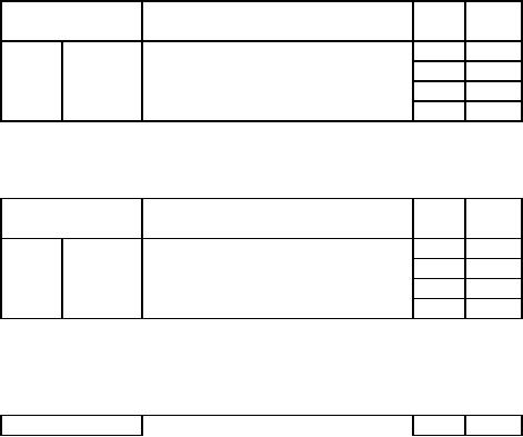
Initial
Table
RHS
Eqn.
Basic
Coefficient
of
Ratio
No.
Variable
S2
S3
Z
x
y
S1
0
-
1
-3
-2
0
0
0
0
40
1
0
1
0
1
0
0
40
40
S1
2
0
0
1
0
1
0
60
∞
S2
3
0
3
2
0
0
1
180
60
S3
First
Iteration: x enters
and S2 leaves the
basis.
RHS
Eqn.
Basic
Coefficient
of
Ratio
No.
Variable
S2
S3
Z
x
y
S1
0
-
1
0
-2
3
0
0
120
1
0
1
0
1
0
0
40
∞
x
2
0
0
1
0
1
0
60
60
S2
3
0
0
2
-3
0
1
60
30
S3
Divide
the equation 3 by to make
key No. 1
Eqn.
Basic
Coefficient
of
RHS
Ratio
149
Operations
Research (MTH601)
150
No.
Variable
Z
x
y
S1
S2
S3
0
-
1
0
-2
3
0
0
120
1
0
1
0
1
0
0
40
x
2
0
0
1
0
1
0
60
60
S2
3
0
0
1
-3/2
0
1/2
30
30
S3
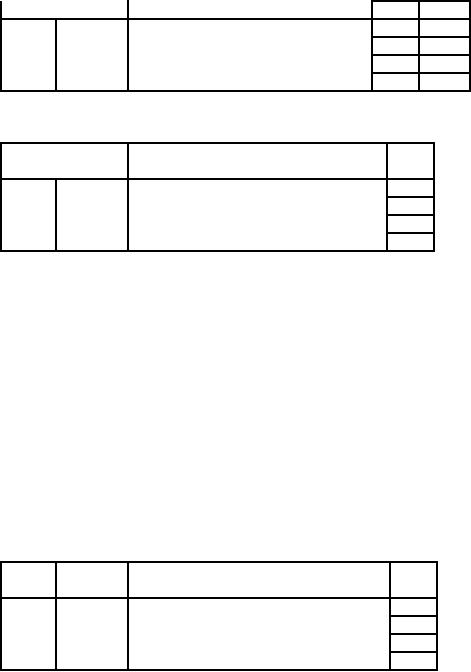
Second
Iteration: y enters
and S3 leaves the
basis.
RHS
Eqn.
Basic
Coefficient
of
No.
Variable
S2
S3
Z
x
y
S1
0
-
1
0
0
0
0
1
180
1
0
1
0
1
0
0
40
x
2
0
0
0
3/2
1
-1/1
30
S2
3
0
0
1
-3/2
0
1/2
30
y
With
this iteration we reach the
optimal solution which is
x
=
40, y
=
3o, S2 = 30, S1 = S3 = 0, Z*
=
180
Now
what is the clue that the
problem has other optimal
solutions?
We
note from the second
iteration that one of the
non-basic variables, S1, has a zero coefficient in
the
current
objective row, representing
Z
=
180 + 0 S1 - S3. Now as the non-basic
variable S1 is increased, the value of
Z
neither
increases nor decreases so
that the corresponding basic
feasible solution should also be
optimal.
We
can find another optimal
basic feasible solution by bringing the
non-basic variable S1 into the basis
and
th
variable S2 leaves the basis. We
have another iteration performed as
shown below.
Third
iteration: S1 enters and
S2 leaves the
basis.
RHS
Eqn.
Basic
Coefficient
of
No.
Variable
S2
S3
Z
x
y
S1
0
1
0
0
0
0
-2
1
180
1
0
1
0
0
-2/3
1/3
20
x
2
0
0
0
3/2
1
-1/2
30
S1
3
0
0
1
0
1
0
60
y
Hence
x
=
20, y
=
60, S1 = 20, S2 = S3 = 0 is another optimal
basic feasible solution.
Still another
iteration
can
also be performed, as the
current objective row has a
zero coefficient for a non-basic
variable. So we conclude
that
we have only two optimal
basic feasible solutions for
the problem. However, any
weighted average of
optimal
solutions
must also be optimal
non-basic feasible solutions.
Indeed there are infinite
numbers of such
solutions,
corresponding
to the points on the line
segment between the two
optimal extreme
points.
150
Operations
Research (MTH601)
151
The
same idea can also be
checked by counting the
number of zero coefficients in the
objective row in
the
optimal table. In all linear
programming problems employing simplex
method, there will be as
many zero
coefficients
in the objective row as
there are basic variables.
But if we find that the
optimal table contains more
zero
coefficients
in the objective row than
the number of variables in
the basis, this is a clear indication
that there will be
yet
another optimal basic
feasible solution.
Non-existing
feasible solution
This
happens when there is no point in
the solution space satisfying all
the constraints. In this
case the
constraints
may be contradictory or there may be
inconsistencies among the
constraints. Thus the
feasible solution
space
is empty and the problem
has no feasible graphical
approach and then by the
simplex method.
Example
(no
feasible solution)
Maximize
Z
=
3x
=
4y
Subject
to
2x +
y
<
12
x
+
2y
>
12
x,
y
>
0
Introduce
slack variables and
artificial variable (for the
constraint of the type >
).
Solution:
We
have the standard form
as
Z
-
3x
-
4y
=0
2x +
y
+
S1
=4
x
+
2y
-
S2 + A
=
12
Since
artificial variable is introduced in
the last constraint, a
penalty of +
MA is
added to the L.H.S
of
the
objective
row. Hence the objective
function equation becomes,
Z
-
3x
-
4y
+ MA =
0
Again
the objective function should
not contain the coefficients of
basic variable. Thus we
multiply the last
constraint
with (-M)
and add to the above
equation. Thus we
have,
Z
-
3x
-
Mx
-
4y
-
2My
+
MS2 = -12M
as
the objective function
equation.
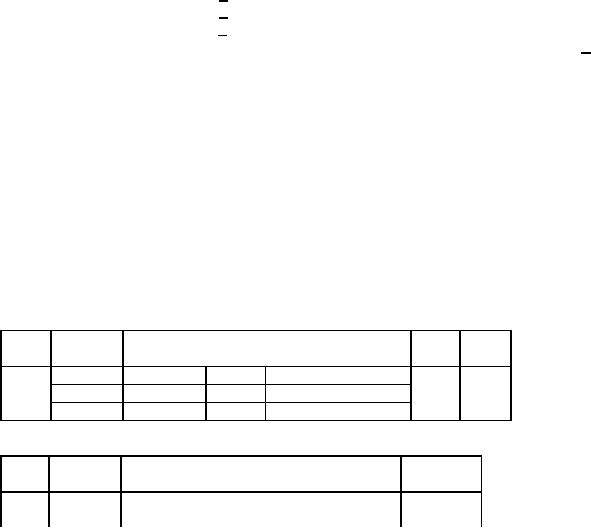
Starting
Table
RHS
Ratio
Eq.
Basic
Coefficient
of
No.
Variable
S2
A
Z
x
y
S1
0
-
1
-M-3
-2M-4
0
0
-12M
M
1
0
2
1
1
0
0
4
4
S1
2
0
1
2
0
-1
1
12
6
A
First
Iteration: y enters
and S1 leaves the
basis.
RHS
Eq.
Basic
Coefficient
of
No.
Variable Z
S2
A
x
y
S1
0
-
1
-
2M+4
0
-4M+16
0
M
3M+5
151
Operations
Research (MTH601)
152
1
0
2
1
1
0
0
4
y
2
0
-3
0
-2
-1
1
4
A
The
last iteration reveals that
we cannot further proceed
with maximization as there is no
negative
coefficient
in the objective function row,
but the final solution has
the artificial variable in
the basis with value at
a
positive
level (equal to 4). This is the
indication that the second
constraint is violated and hence
the problem has no
feasible
optimal solution.
Therefore
a linear programming problem
has no feasible optimal solution if an
artificial variable appears
in
the
basis in the optimal
table.
Unrestricted
Variables
Thus
far we have made the
restrictions for the
decision variables to be non-negative in
most of the practical
or
real life problems. But
there may be situations in
which this is not always the
case. However, the simplex
method
assumes
non-negative variables. But if
the problem involves variables
with unrestricting in sign
(the variables can
take
positive or negative or zero value),
the problem can be converted
into an equivalent one
involving only non-
negative
variables.
A
variable unrestricted in sign
can always be expressed as the
difference of two non-negative
variables. If x
is
the variable unrestricted in
sign, the same can be
replaced with two other
variables say m
and
n
which
are non-
negative
( > 0 ). Thus we have
x=m-n
and
since m and n are
non-negative, the value of x
will be positive if m
n,
negative if m
n and
zero if m
= n.
Thus
the
values of m and n, which are
non-negative, will decide
the fate of the variable
x.
Since the simplex
method
examines
the basic feasible solutions
(extreme points), it will always
have atleast one of these
two no-negative
variables
set equal to zero.
To
illustrate we consider the following
example.
Example
Maximize
Z
= 2x + 5y
Subject
to
<4
x
y
<3
x+y <6
y
>0
Note
that only y
is
non-negative and no mention is
made about x.
Hence x
has
to be treated as a
Solution:
variable
unrestricted in sign. It can
take any value positive,
negative or zero.
Let
x=m-n
Then
we have an equivalent problem by
replacing x
by
(m
- n),
Maximize
Z
=
2m
-
2n
+
5y
152
Operations
Research (MTH601)
153
Subject
to
<4
m-n
y
<3
m-n+y
<6
m,
n, y >
0
Introduce
slack variables and express
the problem in the standard
form. We have
Z
-
2m
+
2n
-
5y
=0
(0)
m-
n
+
S1
=4
(1)
+
S2
=3
(2)
y
m-
n+
y
+
S3
=6
(3)
Starting
Table:
RHS
Ratio
Eq.
Basic
Coefficient
of
No.
Variable
S2
S3
Z
m
n
y
S1
0
-
1
-2
2
-5
0
0
0
0
1
0
1
-1
0
1
0
0
4
∞
S1
2
0
0
0
1
0
1
0
3
3
S2
3
0
1
-1
1
0
0
1
6
6
S3
First
Iteration: y enters
and S2 leaves the
basis.
RHS
Ratio
Eq.
Basic
Coefficient
of
No.
Variable
S2
S3
Z
m
n
y
S1
0
-
1
-2
2
0
0
5
0
15
1
0
1
-1
0
1
0
0
4
4
S1
2
0
0
0
1
0
1
0
3
∞
y
3
0
1
-1
0
0
-1
1
3
3
S3
Second
Iteration: m enters
and S3 leaves the
basis.
RHS
Eq.
Basic
Coefficient
of
No.
Variable
S2
S3
Z
m
n
y
S1
0
-
1
0
0
0
0
3
2
21*
1
0
0
0
0
0
1
-1
1
S1
2
0
0
0
1
0
1
0
3
y
3
0
1
-1
0
0
-1
1
3
m
Therefore
the solution to the original problem
will be
153

Operations
Research (MTH601)
154
Z*
=
21
x=m-n=3
y=3
S1 = 1 and S2 = S3 = 0
If
the original problem has
more than one variable
which is unrestricted in sign,
then the procedure
systematized by
replacing
each such unrestricted
variable xi by xj = mj - n
where
mj > 0 and n
>
0, as before, but n is the
same
variable
for all relevant j.
REVIEW
QUESTIONS
Solve
the Following Problems by
the Simplex
Method
6.
Use
the simplex method to
demonstrate that
the
following problem has an
unbounded optimal
1.
Minimize
solution.
Z
=
2x
+
y
Subject
to
Maximize
x
+
4y
<
1
Z
=
4x1 + x2 + 3x3 + 5x4
x
+
2y
>
4
Subject
to
-4x1 + 6x2 + 5x3 - 4x4 < 20
x,
y
>
0
3x1 - 2x2 + 4x3 + x4 < 10
2.
Maximize
8x1 - 3x2 + 3x3 + 2x4 < 20
Z
=
4x1 + 2x2 + x3
Subject
to
x1, x2, x3, x4 > 0
x1 + x2 < 1
7.
How
do you identify multiple
solutions in a
x1 + x3 < 1
linear
programming problem
using simplex
x1,x2,x3 > 0
procedure?
3.
Maximize
Z
= 4x1 + 3x2
b)
Maximize
Subject
to
Z
=
3x1 + 2x2
4x1 + 2x2 < 10
Subject
to
x1 < 4
6x1 + 8x2 < 24
x2 < 6
3x1 + 2x2 < 18
x1 > 0, x2 > 1.8
x1, x2 > 0
4.
Maximize
8.
Maximize
Z
=
3x1 + x2
Z
=
5u
+
6v
Subject
to
2x1 + x2 > 4
Subject
to
3u + v
<
1
x2 > 2
3u +
4v
<
0
5.
Maximize
Z
=
2x1 + 3x2 + 5x3
and
u
and
v
are
unrestricted.
Subject
to
3x1 + 10x2 + 5x3 15
33x1 - 10x2 + 9x3 < 33
x1 + 2x2 + x3 > 4
x1, x2, x3 > 0
154
Operations
Research (MTH601)
155
DUALITY
THEORY
For
every linear programming
problem, there is an associated
linear programming problem
and if the
former
problem is called the primal
linear programming problem
the latter is called its
dual and vice versa.
The
concept
of duality was also
developed along with the
linear programming discovery. It has
many important
ramifications.
The two problems may
appear to have only superficial
relationship between each
other, but they
possess
very intimately related
properties and useful one,
so that the optimal solution of
one problem gives
complete
information
about the optimal solution to
the other.
We
shall present later a few
examples to illustrate how these
relationships are useful in
reducing
computational
effort while solving the linear
programming problems. This concept of
duality is very much useful
to
obtain
additional information about the
variations in the optimal solution
when certain changes are
effected in the
constraint
coefficients, resource availabilities and
objective function coefficients. This is
termed as post-optimality
or
sensitivity analysis.
Dual
Formulation
The
following procedure is generally
adopted to convert the
primal linear programming
problem to its dual.
STEP
1 For
each constraint in primal
problem there is an associated
variable in the dual
problem.
STEP
2 The
elements of the right hand
side of the constraints in
the primal problem are
equal to the
respective
coefficients
of the objective function in the
dual problem.
STEP
3 When
primal problem seeks
maximization as the measure of
effectiveness the dual
problem seeks
minimization
and vice versa.
STEP
4 The
maximization problem has
constraints of type (< ) and
the minimization problem has
constraints of the
type
( > ).
STEP
5 The
variables in both the
problems are non-negative
(sometimes unrestricted).
STEP
6 The
rows of the primal problem
are changed to columns in
the dual problem.
Example
Maximize
Z
=
6x1 + 7x2 + 8x3
Subject
to
x1 + 2x2 + 7x3 < 60
2x1
+
3x3 < 20
4x2 + 5x3 < 45
x3 < 15
x1, x2, x3 > 0
We
consider the given problem
as the primal linear
programming problem. To convert
into dual,
Solution:
the
following procedure is
adopted.
155
Operations
Research (MTH601)
156
STEP
1 We
have four constraints in the
primal problem. So we choose four
dual variables, say
y1, y2, y3 and y4.
Connect
these variables with the
right hand side of each
constraint, respectively.
STEP
2 The
primal objective function is one of
maximization. Hence, the
dual seeks minimization for
the objective
function.
The right hand side of the
primal problem is associated
with the respective dual
variable and written
as
Minimize
Z
=
60y1 +20y2 + 45y3 + 15y4
STEP
3 Considering
the primal problem, the
matrix formed with
constraint coefficients as elements in
the matrix is
transposed
and the elements of
transposed matrix will be coefficients of
constraints for the dual
problem. Note that
the
constraints in the primal
problem are of the type (
< ). If any of the constraint is of
the type ( > ) in a
maximization
problem convert into ( < ) inequality
by multiplying the constraint
throughout by (-1). In a
minimization
problem convert the inequality of
the type ( < ) into ( > ) by
multiplying the constraint
by(-1).
⎡1
2
7⎤
⎢2
0
3⎥
In
the above problem we have
the coefficient matrix as ⎢
⎥
⎢0
45
⎥
⎢0
0
1⎥
⎣
⎦
⎡1
2 0 0⎤
⎢2
0 4 0⎥
The
transpose of the above
matrix is
⎢7
3 5 1⎥
⎣
⎦
STEP
4 Treat
the above elements as the
coefficients for the constraints of
the dual and the
objective coefficient of
the
primal variables are taken
as the right hand side
for the constraints in the
dual problem.
STEP
5 The
dual problem seeks
minimization and hence the
constraints of the dual
problem will have inequality
of
the
type ( > ).
Hence
we have the dual for
the problem as
follows:
Minimize
Z
=
60y1 +20y2 +45y3 +15y4
Subject
to
y1 + 2y2
>6
2y1
4y3
>7
7y1 +3y2 + 5y3 + y4 > 8
y1,
y2, y3, y4 > 0
The
Constraints having equality
sign
An
equality constraint in the primal
problem corresponds to an unrestricted
variable in sign in the
dual
problem
and vice versa. To illustrate consider
the example.
156
Operations
Research (MTH601)
157
Example
Maximize
Z
=
c1x1 + c2x2
Subject
to
a11x1 + a12x2 = b1
a21x1 + a22x2 < b2
x1,
x2 > 0
The
first constraint has the
equality sign. Hence this
can be replaced by two
equivalent constraints taken
together as
a11x1 + a12x2 < b1
and
a11x1 + a12x2 > b1
or
the same can be written
as
a11x1 + a12x2 < b1
and
-a11x1 - a12x2 < -b1
+
-
Let
y1 , y1 and y2 be the dual variables
corresponding to the primal
problem.
Thus
the dual problem is
(
)
+b
y
+
-
Z
=
b1 y1 -
y1
Minimize
2 2
(
)
+a
+
-
a11 y1 -
y1
>
c1
Subject
to
21y2
(y
)
+a
+
-
-
y1
>
c2
a12
22y2
1
+
-
y1 , y1 and y2 > 0
and
(y
)
is
observed in the objective function
and all the constraints.
This will be the case
+
-
-
y1
The
term
1
whenever
there is an equality constraint in the
primal. So if we replace (
y
-
y
) by
a new variable y
which
is the
+
-
1
1
1
difference
between two non-negative
variables, the variable
y1 will become unrestricted
in sign and the dual
problem
the
variable y1 will become unrestricted
in sign and the dual
problem is
Minimize
Z
=
b1 y1 + b2 y2
Subject
to
a11y1 + a21y2 > c1
a12y1 + a22y2 > c2
y1 is unrestricted in
sign
y2 > 0
Thus
we must have the dual
variable corresponding to the equality
constraint unrestricted in
sign.
157
Operations
Research (MTH601)
158
Conversely,
when a primal variable is
unrestricted in sign, its
dual constraint must be
expressed as an equation.
The
following examples reveal
the conversion of the primal
problem into dual.
Example
Write
the dual of the following
problem.
Maximize
Z
=
-6x1 + 7x2
Subject
to
-x1 + 2x2 < -5
3x1 + 4x2 < 7
x1, x2 > 0
Solution:
There
are two constraints.
Therefore we have two dual
variables y1 and y2. Then we have the
dual as
follows:
Minimize
Z
=
-5y1 + 7y2
Subject
to
-y1 + 3y2 > -6
2y1 + 4y2 > 7
y1, y2 > 0
Example
Write
the dual of the
problem
Minimize
Z
=
5x1 + 2x2
Subject
to
6x1 - 2x2 + 2x3 > 20
2x1 + 4x2 + x3 > 40
x1, x2, x3 > 0
Solution
Note
that the objective function
has coefficient 0 for x3.
Maximize
Z
=
20y1 + 40y2
Subject
to
6y1 + 2y2 < 5
-2y1 + 4y2 < 2
2y1 + y2 < 0
y1, y2 > 0
Example
Write
the dual of the
problem
Maximize
Z
=
2x1 + x2 + 13x3 - 5x4
Subject
to
-x1 + x2 + x3 - x4 = 15
6x1 + 5x2 - 7x3 + 2x4 > 18
10x1 - 8x2 + 2x3 + 4x4 < 25
x1, x2,
x4 > 0
x3 is unrestricted.
158

Operations
Research (MTH601)
159
Solution:
Before
converting the problem into
dual the following
observations are made
regarding the primal
problem.
1.
The
objective function seeks maximization.
Hence the constraints must
be expressed as ( < ) type.
The
second constraint is of the
type ( > ). It has to be converted
into ( < ) bye multiplying
throughout the
constraint
by (-1).
i.e.,
-6x1 - 5x2 + 7x3 - 2x4 < -18
2.
The
first primal constraint has
equality sign. Hence the
corresponding dual variable
will be
unrestricted
in sign and the third
primal variable is unrestricted
and so the corresponding third
dual
constraint
will be an equation.
Minimize
Z
=
15y1 - 18y2 + 25y3
-y1 - 6y2 + 10y3 > 2
y1 - 5y2 - 8y3 > 1
y1 + 7y2 + 2y3 = 13
-y1 - 2y2 + 4y3 > -5
y1 is unrestricted
y2, y3 > 0
Example
Write
the dual to the following
problems, solve the dual
and hence find the solution
to the primal problem
from
the results of the
dual.
Minimize
Z
=
4x1 + 3x2 + 6x3
Subject
to
x1 +
x3 > 2
x2 + x3 > 5
x1 , x2 , x3 > 0
Solution
The
dual for the given
problem can be easily
written as
Minimize
Z
=
2y1+ 5y2
Subject
to
<4
y1
y2 < 3
y1 + y2 < 6
y1 , y2 > 0
(Note
that it is easier to solve
the dual problem than
the primal since the
primal problem involves the
use of artificial
variable
technique and it may lead to
tedious calculations.)
Introducing
the slack variable for
the constraints, we
have
Z
-
2y1 - 5y2 = 0
(0)
y1 + S1 = 4
(1)
y2 + S2 = 3
(2)
y1+y2+S3 = 6
(3)
159
Operations
Research (MTH601)
160
Starting
table
RHS
Ratio
Eq.
Basic
Coefficient
of
No.
Variable
y2
S1
S2
S3
Z
y1
0
-
1
-2
-5
0
0
0
0
1
0
1
0
1
0
0
4
∞
S1
2
0
0
1
0
1
0
3
3
S2
3
0
1
1
0
0
1
6
6
S3
First
Iteration: y2 enters and
S2 leaves the
basis.
RHS
Ratio
Eq.
Basic
Coefficient
of
No.
Variable
y2
S1
S2
S3
Z
y1
0
-
1
-2
0
0
5
0
15
1
0
1
0
1
0
0
4
4
S1
2
0
0
1
0
1
0
3
∞
y2
3
0
1
0
0
-1
1
3
3
S3
Second
Iteration: y1 enters and
S3 leaves the
basis.
RHS
Eq.
Basic
Coefficient
of
No.
Variable
y2
S1
S2
S3
Z
y1
0
-
1
0
0
0
3
2
21*
1
0
0
0
1
1
-1
1
S1
2
0
0
1
0
1
0
3
y2
3
0
1
0
0
-1
1
3
y1
The
optimal solution to the dual
problem as seen from the
last table is
Z*
=
21; y1 = 3, y2 = 3, S1 = 1, S2 = S3 = 0
The
solution to the primal problem
can be obtained from the
optimal table of the dual
problem by
identifying
the coefficients of those variables in
the objective row of the
optimal table which have
been taken as the
basic
variables in the starting
table of the dual
problem.
In
the above example, the
variables, S1, S2 and S3 have been chosen to
form the basis in the
starting table of
the
dual. The corresponding
coefficients of the same
variables S1, S2 and S3 in the objective row of
the optimal table
are
0, 3 and 2 respectively and
these are the optimal
values of the variables in
the primal problem
namely,
x1 = 0
x2 = 3
x3 = 2
Note
that the objective function
has the same value in both
primal and dual problems.
160
Operations
Research (MTH601)
161
The
primal optimal solution is
Z*
=
21, x1 = 0, x2 = 3 and x3 = 2.
Economic
Interpretation of the Dual
The
duality concept has a
natural economic interpretation,
which is useful for economic
analysis. We know
that
the linear programming
problem is mainly concerned
with the allocation of scarce
resources among many
activities
in competition.
If
xj is the level of activity
j,
cj is the unit profit
from activity expressed in
rupees,
bi is
the amount of resource
i
available,
aij is
the amount of resource
i
consumed
by each unit of activity
j,
then
consider a constraint from
the corresponding dual
problem.
a1j y1
+ a2jy2
+ ... +
amj ym
> cj
We
have from the primal
problem, the unit of
Cj is in
rupees per unit of activity
j
and
the units of aij are
the units of
resource
i
per
unit of activity j.
This implies that yi must have units of
rupees per unit of resource
i.
In other words, yi
may
be interpreted as the unit prices of
resource i
in
the sense of implicit or
imputed value of the
resource to the
i=m
∑
aij yi
user.
Also,
can
also be interpreted as the
imputed cost of operating
activity j
at
unit level.
i
=1
i=m
∑
aij yi
≥
c j suggests
that this imputed cost
should not be less than
the profit, which
could
The
inequality,
i
=1
i=m
Z
y = ∑
bi yi
be
achieved from the activity.
The dual objective
i
=1
indicates
that the prices of the
resources should be set so as to
minimize their total cost.
The optimal value of
the
dual
variables, yi*
(i =
1, 2, ..., m)
then represents the
incremental value, or shadow
theorem Zx*
=
Zy*
implies
that
the
total cost (implicit value) of
the resources equals the
total profit from the
activites using them in an
optimal
manner.
It
is interesting to note that
the interpretation of yi*
developed above is the rate
at which the profit
would
change
(increase or decrease) when
the amount of resource
i
is
changed (increased or decreased)
over a certain
range
of bi over
which the original optimal
basis is not changed. In
fact y1*
does
represent the marginal value
of
resource
i.
Applications
of Duality
(a)
From
the theorems of duality we
understand that solving either
primal or the dual
problem
automatically
solves the other problem. So
we can apply simplex method
to the problem requiring
less
computational
effort, if we want to identify the
optimal primal solution. The
time consumed in a computer in
using
the
simplex method is quite
sensitive to the number of
constraints. We also know
that the number of
original
161
Operations
Research (MTH601)
162
variables
in the primal problem is
equal to the number of
constraints in the dual
problem whenever the
original
form
of primal problem has more
constraints than variables
(m
n).
(b)
Another important application of
concept of duality is to the
analysis of the problem if
the parameters
are
changed after the original
optimal solution has been
obtained. This is normally dealt in
the topic 'duality and
post
optimality
analysis'.
(c)
In duality analysis, we know
that the value of the
objective function for any
feasible solution of the
dual
problem provides an upper
bound to the optimal value
of the objective function for
the primal problem.
This
concept
is useful to get an idea of
how well or how much
better one can do by
expending the effort needed to
obtain
the
primal solution.
To
illustrate, consider the following
primal linear programming
problem.
Maximize
Zx =
3x1 + 4x2
Subject
to
x1 < 3
x2 < 4
x1 + x2 < 5
and
x1, x2 > 0
The
dual of the above problem
can be written as
Minimize
Zy =
3y1 + 4y2 + 5y3
Subject
to
y1 + y3 > 3
y2 + y3 > 4
and
y1, y2, y3 > 0
If
we assume feasible values of
y1 = 3, y2 = 4 and y3 = 0, the objective function
value Zy = 3y1 + 4y2 + 5y3 =
25.
So, without further
investigation, it will be clear
that Zx = 25.
In fact the maximum value
Zx* = 17 as
obtained by
simplex
method.
REVIEW
QUESTIONS
1.
Find
the dual of the following
Problems
(a)
Maximize
Where
x1 + 3x2
x1 > 0, x2 > 0
and
x1 + 2x2 < 10
Subject
to
6x1 + 19x2 < 100
-x1 - x2 < 30
3x1 + 5x2 < 40
x1 - 3x2 < 33
(c)
Maximize
2x1 + x2 + x3 - x4
x2 < 25
x1 < 42
Subject
to
x1,
x2 > 0
x1 - x2 + 2x3 + 2x4 < 3
2x1 + 2x2 -x3
=4
x1 - 2x2 + 3x3 + 4x4 > 5
(b)
Maximize
P
=
x1 + 2x2
x1 - 2x2 + 3x3 + 4x4 > 5
x1, x2, x3 > 0
162
Operations
Research (MTH601)
163
x4 unrestricted.
(d)
Maximize
x0 = 15x1 + 3x2 + 16x3
x1 + x2 - x3 + 2x4 < 2
x1 + x2 - x3
<2
x1 + 13x2 + x3
=2
x1,
x2, x3
>0
(e)
Maximize
4x1 + 5x2 + 3x3 + 6x4
Subject
to
x1 + 3x2 + x3 + 2x4 < 2
3x1 + 3x2 + 2x3 +2x4 < 4
3x1 + 2x2 + 4x3 + 5x4
< 6
x1, x2, x3, x4 > 0
(f)
Maximize
Z
=
x1 + 1.5x2
Subject
to
2x1 + 3x2 < 25
x1 + x2 > 1
x1 - 2x2 = 1
x1 , x2 > 0
(g)
Maximize
x0 = 2x1 + 3x3
Subject
to
-3x1 + x2 + 2x3 < 5
-2x1 - x2
<1
x1, x2, x3
>0
163
Table of Contents:
- Introduction:OR APPROACH TO PROBLEM SOLVING, Observation
- Introduction:Model Solution, Implementation of Results
- Introduction:USES OF OPERATIONS RESEARCH, Marketing, Personnel
- PERT / CPM:CONCEPT OF NETWORK, RULES FOR CONSTRUCTION OF NETWORK
- PERT / CPM:DUMMY ACTIVITIES, TO FIND THE CRITICAL PATH
- PERT / CPM:ALGORITHM FOR CRITICAL PATH, Free Slack
- PERT / CPM:Expected length of a critical path, Expected time and Critical path
- PERT / CPM:Expected time and Critical path
- PERT / CPM:RESOURCE SCHEDULING IN NETWORK
- PERT / CPM:Exercises
- Inventory Control:INVENTORY COSTS, INVENTORY MODELS (E.O.Q. MODELS)
- Inventory Control:Purchasing model with shortages
- Inventory Control:Manufacturing model with no shortages
- Inventory Control:Manufacturing model with shortages
- Inventory Control:ORDER QUANTITY WITH PRICE-BREAK
- Inventory Control:SOME DEFINITIONS, Computation of Safety Stock
- Linear Programming:Formulation of the Linear Programming Problem
- Linear Programming:Formulation of the Linear Programming Problem, Decision Variables
- Linear Programming:Model Constraints, Ingredients Mixing
- Linear Programming:VITAMIN CONTRIBUTION, Decision Variables
- Linear Programming:LINEAR PROGRAMMING PROBLEM
- Linear Programming:LIMITATIONS OF LINEAR PROGRAMMING
- Linear Programming:SOLUTION TO LINEAR PROGRAMMING PROBLEMS
- Linear Programming:SIMPLEX METHOD, Simplex Procedure
- Linear Programming:PRESENTATION IN TABULAR FORM - (SIMPLEX TABLE)
- Linear Programming:ARTIFICIAL VARIABLE TECHNIQUE
- Linear Programming:The Two Phase Method, First Iteration
- Linear Programming:VARIANTS OF THE SIMPLEX METHOD
- Linear Programming:Tie for the Leaving Basic Variable (Degeneracy)
- Linear Programming:Multiple or Alternative optimal Solutions
- Transportation Problems:TRANSPORTATION MODEL, Distribution centers
- Transportation Problems:FINDING AN INITIAL BASIC FEASIBLE SOLUTION
- Transportation Problems:MOVING TOWARDS OPTIMALITY
- Transportation Problems:DEGENERACY, Destination
- Transportation Problems:REVIEW QUESTIONS
- Assignment Problems:MATHEMATICAL FORMULATION OF THE PROBLEM
- Assignment Problems:SOLUTION OF AN ASSIGNMENT PROBLEM
- Queuing Theory:DEFINITION OF TERMS IN QUEUEING MODEL
- Queuing Theory:SINGLE-CHANNEL INFINITE-POPULATION MODEL
- Replacement Models:REPLACEMENT OF ITEMS WITH GRADUAL DETERIORATION
- Replacement Models:ITEMS DETERIORATING WITH TIME VALUE OF MONEY
- Dynamic Programming:FEATURES CHARECTERIZING DYNAMIC PROGRAMMING PROBLEMS
- Dynamic Programming:Analysis of the Result, One Stage Problem
- Miscellaneous:SEQUENCING, PROCESSING n JOBS THROUGH TWO MACHINES
- Miscellaneous:METHODS OF INTEGER PROGRAMMING SOLUTION