Issues of Dimensional Modeling: Additive vs Non-Additive facts, Classification of Aggregation Functions

<< Process of Dimensional Modeling: Four Step: Choose Business Process, Grain, Facts, Dimensions

Extract Transform Load ETL: ETL Cycle, Processing, Data Extraction, Data Transformation >>

Lecture-15

Issues of Dimensional Modeling

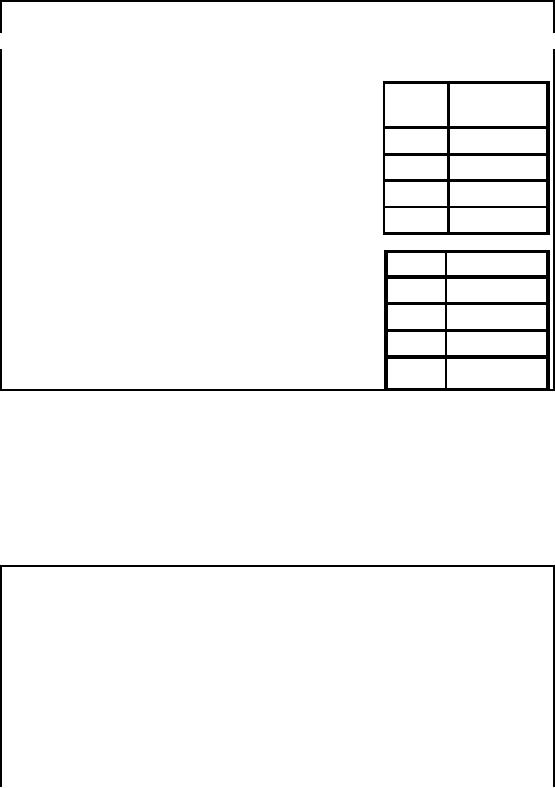
Step 3: Additive vs. Non-Additive facts

Additive facts are easy to work with

Month

Crates of

§ Summing the fact value gives

Bottles Sold

meaningful results

§ Additive facts:

May

§ Quantity sold

Jun.

§ Total Rs. sales

Jul.

Non-additive facts:

§ Averages

(average

TOTAL

sales price, unit price)

§ Percentages

Month

% discount

discount)

§ Ratios (gross margin)

May

§ Count of distinct

products sold

Jun.

Jul.

TOTAL 24%

Incorrect!

There can be two types of facts i.e. additive and non-additive. Additive facts are those facts which

give the correct result by an addition operation. Examples of such facts could be number of items

sold, sales amount etc. Non-additive facts can also be added, but the addition gives incorrect

results. Some examples of non-additive facts are average, discount, ratios etc. Consider three

instances of 5, with the sum being 15 and average being 5. Now consider two numbers i.e. 5 and

10, the sum being 15, but the average being 7.5. Now if the average of 5 and 7.5 is taken this

comes to be 6.25, but if the average of the actual numbers is taken, the sum comes to be 30 and

the average being 6. Hence averages, if added gives wrong results. Now facts could be averages,

such as average sales per week etc, thus they are perfectly legitimate facts.

Step-3: Classification of Aggregation Functions

How hard to compute aggregate from sub-aggregates?

Three classes of aggregates:

Distributive

§ Compute aggregate directly from sub-aggregates

§ Examples: MIN, MAX ,COUNT, SUM

Algebraic

§ Compute aggregate from constant-sized summary of subgroup

§ Examples: STDDEV, AVERAGE

§ For AVERAGE, summary data for each group is SUM, COUNT

108

Holistic

§ Require unbounded amount of information about each subgroup

§ Examples: MEDIAN, COUNT DISTINCT

§ Usually impractical for a data warehouses!

We see that calculating aggregates from aggregates is desirable, but is not possible for non -

additive facts. So we deal with three types of aggregates i.e. distributive that are additive in

nature, and then algebraic which are non-additive in nature. Therefore, such aggregates have to be

computed from summary of subgroups to avoid the problem of incorrect results. The of course

are the holistic aggregates that give a complete picture of the data, such as median, or distinct

values. However, such aggregates are not desirable for a data warehouse environment, as it

requires a complete scanning, which is highly undesirable as it consumes lot of time.

Step-3: Not recording Facts

Transactional fact tables don't have records for events that don't occur

§ Example: No records(rows) for products that were not sold.

This has both advantage and disadvantage.

§ Advantage:

§ Benefit of sparsity of data

§ Significantly less data to store for "rare" events

Disadvantage: Lack of information

Example: What products on promotion were not sold?

Fact tables usually don't records events that don't happen, such as items that were not sold. The

advantage of this approach is getting around the problem of sparsity. Recall that when we

discussed MOLAP, we discussed the sales of different items not occurring in different

geographies and in different time frames, resulting in sparse cubes. If however this data is not

recorded, then significantly less data will be required to be stored. But what if, from the point of

view of decision making, such data has to be retrieved, how to retrieve data corresponding to

those items? To find such items, additional queries will be required to check the current item

balance with the item balance when the items where (say) brought into the store. So the biggest

disadvantage of this approach is key data is not recorded.

Step-3: A Fact-less Fact Table

"Fact -less" fact table

§ A fact table without numeric fact columns

Captures relationships between dimensions

Use a dummy fact column that always has value 1

The problem of not recording non-events is solved by using fact -less fact tables, as not recording

such information resulted in loss of data. Such a fact -less fact table is one which does not have

numeric values stored in the corresponding column, as such tables are used to capture the

relationships between dimensions. Fact less fact table captures the many-to-many relationships

109

between dimensions, but contains no numeric or textual facts. To achieve this dummy value of 1

is used in the corresponding column.

Step-3: Example: Fact-less Fact Tables

Examples:

Department/Student mapping fact table

What is the major for each student?

Whi ch students did not enroll in ANY course

Promotion coverage fact table

Which products were on promotion in which stores for which days?

Kind of like a periodic snapshot fact

Some of the examples of fact -less fact tables. Consider the case of a department/student mapping

fact table. The data is recorded for each student who registers for a course, but there may be

students that do not register in any course. If data is useful from the point of view of identifying

those students which are skipping a semester. There is no direct or simple way to identify such

students, the solution is a fact -less fact table. Similarly which items on promotion are not selling,

as the sales records are for only those items that are sold.

Step-4: Handling Multi-valued Dimensions?

One of the following approaches is adopted:

Drop the dimension.

Use a primary value as a single value.

Add multiple values in the dimension table.

Use "Helper" tables.

For handling the exceptions in dimensions, designers adopt one of the following approaches:

Drop the Maintenance_Operation dimension as it is multi-valued.

Choose one value (as the "primary" maintenance) and omit the other values.

Extend the dimension list and add a fixed number of maintenance dimensions.

Put a helper table in between this fact table and the Maintenance dimension table.

Instead of ignoring the problem and dropping the dimension altogether, let's tackle the problem.

Usually the designers go for the second alternative, as a consequence this will show up as the

primary, or main maintenance operation. Such as 20,000 Km maintenance or 40,000 Km

maintenance. It is known what would constitute for each mileage based maintenance, and these

maintenance are also mutually exclusive i.e. single valued. In many cases , you may actually come

110

across this practice being observed in the OLTP systems. The obvious advantage is that the

modeling problem is resolved, but the disadvantage is that the usefulness of the data becomes

questionable. Why? Because with the passage of time or with new models of vehicles coming or

because of company policy, what constitutes service at 20,000 Km may actually change. Will

need meta data to resolve this issue.

The third alternative of creating a fixed number of additional columns in the dimension table is a

quick and dirty approach and should be avoided. There is likely to be car that may require more

changes then reflected in the table, or the company policy changes and more items fall under the

maintenance, and a long list will result i n many null entries for a typical car, especially new ones.

Furthermore, it is not easy to query the multiple separate maintenance dimensions and will result

in slow queries. Therefore, multiple dimensions style of design should be avoided.

The last alternative is usually adopted, and a "helper" table is placed between the Maintenance

dimension and the fact table, although this adulterates or dilutes the star schema. More details are

beyond the scope of this course.

Step-4: OLTP & Slowly Changing Dimensions

OLTP systems not good at tracking the past. History never changes.

OLTP systems are not "static" always evolving, data changing by overwriting.

Inability of OLTP systems to track history, purged after 90 to 180 days.

Actually don't want to keep historical data for OLTP system.

One major difference between an OLTP system and a data warehouse is the ability and the

responsibility to accurately describe the past. OLTP systems are usually very poor at correctly

representing a business as of a month or a year ago for several reasons as discussed before. A

good OLTP system is always evolving. Orders are being filled and, thus, the order backlog is

constantly changing. Descriptions of products, suppliers, and customers are constantly being

updated, usually by overwriting. The large volume of data in an OLTP system is typically purged

every 90 t o 180 days. For these reasons, it is difficult for an OLTP system to correctly represent

the past. In an OLTP system, do you really want to keep old order statuses, product descriptions,

supplier descriptions, and customer descriptions over a multiyear period?

Step-4: DWH Dilemma: Slowly Changing Dimensions

The responsibility of the DWH to track the changes.

Example: Slight change in description, but the prod uct ID (SKU) is not changed.

Dilemma: Want to track both old and new descriptions, what do they use for the key? And where

do they put the two values of the changed ingredient attribute?

The data warehouse must accept the responsibility of accurately describing the past. By doing so,

the data warehouse simplifies the responsibilities of the OLTP system. Not only does the data

warehouse relieve the OLTP system of almost all forms of reporting, but the data warehouse

contains special structures that have several ways of tracking historical data.

111

A dimensional data warehouse database consists of a large central fact table with a multipart key.

This fact table is surrounded by a single layer of smaller dimension tables, each containing a

single primary key. In a dimensional database, these issues of describing the past mostly involve

slowly changing dimensions. A typical slowly changing dimension is a product dimension in

which the detailed description of a given product is occasionally adjusted. For example, a minor

ingredient change or a minor packaging change may be so small that production does not assign

the product a new SKU number (which the data warehouse has been using as the primary key in

the product dimension), but nevertheless gives the data wa rehouse team a revised description of t

he product. The data warehouse team faces a dilemma when this happens. If they want the data

warehouse to track both the old and new descriptions of the product, what do they use for the

key? And where do they put the two values of the changed ingredient

Step-4: Explanation of Slowly Changing Dimensions...

Compared to fact tables, contents of dimension tables are relatively stable.

§ New sales transactions occur constantly.

§ New products are introduced rarely.

§ New stores are opened very rarely.

The assumption does not hold in some cases

§ Certain dimensions evolve with time

§ e.g. description and formulation of products change with time

§ Customers get married and divorced, have children, change addresses etc.

§ Land changes ownership etc.

§ Changing names of sales regions.

For example, a minor ingredient change or a minor packaging change may be so small that

production does not assign the product a new SKU number (which the data warehouse has been

using as the primary key in t he product dimension), but nevertheless gives the data warehouse

team a revised description of t he product. The data warehouse team faces a dilemma when this

happens. If they want the data warehouse to track both the old and new descriptions of the

product, what do they use for the key? And where do they put the two values of the changed

ingredient attribute?

Other common slowly changing dimensions are the district and region names for a sales force.

Every company that has a sales force reassigns these names every year or two. This is such a

common problem that this example is something of a joke in data ware housing classes. When the

teacher asks, "How many of your companies have changed the organization of your sales force

recently?" everyone raises their hands.

Step-4: Explanation of Slowly Changing Dimensions...

Although these dimensions change but the change is not rapid.

Therefore called "Slowly" Changing Dimensions

There can be many examples. For a young customer who is single, then after a w ile the

customer gets married. After sometime there are children, in unfortunate cases the marriage

breaks so the customer is separated or the husband dies and the customer becomes a widow. This

just does not typically happen overnight but takes a while. Another example is inheritance,

consider the example of land. Over a period of time the land changes hands, is split because of

112

inheritance or its size increases by buying. Again things don't happen overnight, but take a while,

hence slowly changing dimens ions.

Step-4: Handling Slowly Changing Dimensions

Option-1: Overwrite History

§ Example: Code for a city, product entered incorrectly

Just overwrite the record changing the values of modified attributes.

No keys are affected.

No changes needed elsewhere in the DM.

Cannot track history and hence not a good option in DSS.

The first technique is the simplest and fastest. But it doesn't maintain past history! Nevertheless,

overwriting is frequently used when the data warehouse team legitimately decides that the old

value of the changed dimension attribute is not interesting . For example, if you find incorrect

values in the city and state attributes in a customer record, then overwriting would almost

certainly be used. After the overwrite, certain old reports that depended on the city or state values

would not return exactly the same values. Most of us would argue that this is the correct outcome.

Step-4: Handling Slowly Changing Dimensions

Option-2: Preserve History

Example: The packaging of a part change from glued box to stapled box, but the

code assigned (SKU) is not changed.

Create an additional dimension record at the time of change with new attribute

values.

Segments history accurately between old and new description

Requires adding two to three version numbers to the end of key. SKU#+1,

SKU#+2 etc.

Suppose you work in a manufacturing company and one of your main data warehouse schemas is

the company's shipments. The product dimension is one of the most important dimensions in this

dimensional schema. A typical product dimension would have several hundred detailed records,

each representing a unique product capable of being shipped. A good product dimension table

would have at least 50 attributes describing the products, including hierarchica l attributes such as

brand and category, as well as nonhierarchical attributes such as color and package type. An

important attribute provided by manufacturing operations is the SKU number assigned to the

product. You should start by using the SKU number as the key to the product dimension table.

Suppose that manufacturing operations makes a slight change in packaging of SKU #38, and the

packaging description changes from "glued box" to "pasted box." Along with this change,

manufacturing operations decides not to change the SKU number of the product, or the bar code

(UPC) that is printed on the box. If the data warehouse team decides to track this change, the best

way to do this is to issue another product record, as if the pasted box version were a brand new

113

product. The only difference between the two product records is the packaging description. Even

the SKU numbers are the same. The only way you can issue another record is if you generalize

the key to the product dimension table to be something more than the SKU number. A simple

technique is to use the SKU number plus two or three version digits. Thus the first instance of the

product key for a given SKU might be SKU# + 01. When, and if, another version is needed, it

becomes SKU# + 02, and so on. Notice that you should probably also park t he SKU number in a

separate dimension attribute (field) because you never want an application to be parsing the key

to extract the underlying SKU number. Note the separate SKU attribute in the Product dimension

in Figure 1.

This technique for tracking slowly changing dimensions is very powerful because new dimension

records automatically partition history in the fact table. The old version of the dimension record

points to all history in the fact table prior to the chang e. The new version of the dimension record

points to all history after the change. There is no need for a timestamp in the product table to

record the change. In fact, a timestamp in the dimension record may be meaningless because the

event of interest is t he actual use of the new product type in a shipment. This is best recorded by

a fact table record with the correct new product key.

Another advantage of this technique is that you can gracefully track as many changes to a

dimensional item as you wish. Each change generates a new dimension record, and each record

partitions history perfectly. The main drawbacks of the technique are the requirement to

generalize the dimension key, and the growth of the dimension table itself.

Step-4: Handling Slowly Changing Dimensions

Option-3: Create current valued field

Example: The name and organization of the sales regions change over time, and

want to know how sales would have looked with old regions.

Add a new field called current_region rename old to previous_region.

Sales record keys are not changed.

Only TWO most recent changes can be tracked.

Creating a Current Value Field

You use the third technique when you want to track a change in a dimension value, but it is

legitimate to use the old value both before and after the change. This situation occurs most often

in the infamous sales force realignments, where although you have changed the names of your

sales regions, you still have a need to state today's sales in terms of yesterday's region names, just

to "see how they would have done" using the old organization. You can attack this requirement,

not by creating a new dimension record as in the second technique, but by creating a new "current

value" field. Suppose in a sales team dimension table, where the records represent sales teams,

you have a field called "region." When you decide to rearrange the sales force and assign each

team to newly named regions, you create a new field in the sales dimension table called

"current_region." You should probably rena me the old field "previous_region." No alterations are

made to the sales dimension record keys or to the number of sales team records. These two fields

now allow an application to group all sales fact records by either the old sales assignments

(previous region) or the new sales assignments (current region). This schema allows only the

most recent sales force change to be tracked, but it offers the immense flexibility of being able to

114

state all of the history by either of the two sales force assignment sche mas. It is conceivable,

although somewhat awkward, to generalize this approach to the two most recent changes. If many

of these sales force realignments take place and it is desired to track them all, then the second

technique should probably be used.

S tep-4: Pros and Cons of Handling

Option-1: Overwrite existing value

+ Simple to implement

+ No tracking of history

Option-2: Add a new dimension row

+ Accurate historical reporting

+ Pre-computed aggregates unaffected

+ Dimension table grows over time

Option-3: Add a new field

+ Accurate historical reporting to last TWO changes

+ Record keys are unaffected

+ Dimension table size increases

There are number of ways of handling slowly changing dimensions. Some of the methods are

simple, but not desirable; but all have their own pros and cons. The simplest possible "solution" is

to overwrite history. If the customer was earlier single, and gets married, just change his/here

status from single to married. Very simple to implement, but not desirable, as a DWH is about

recording historical data, and by virtue of overwriting, the historical data is destroyed. Another

option is to add a row when the dimension changes, the obvious benefit is that history is not lost,

but over the period of time the dimension table will grow as new rows are added corresponding to

the changes in the dimensions. The third, rather desirable approach is to add an additional

column, that does increase the table size, but the increase is not non -deterministic. The column

records the last two changes, if the dimension changes more than twice, then historical data is

lost.

Step-4: Junk Dimension

Sometimes certain attributes don't fit nicely into any dimension

§ Payment method (Cash vs. Credit Card vs. Check)

§ Bagging type (Paper vs. Plastic vs. None)

Create one or more "mix" dimensions

§ Group together leftover attributes as a dimension even if not related

§ Reduces number of dimension tables, width of fact table

§ Works best if leftover attributes are

§ Few in number

§ Low in cardinality

§ Correlated

Other options

§ Each leftover attribute becomes a dimension

§ Eliminate leftover attributes that are not useful

115

A junk dimension is a collection of random transactional codes, flags and/or text attributes that

are unrelated to any particular dimension. The junk dimension is simply a structure that provides

a convenient place to store the junk attributes. A good example would be a trade fact in a

company that brokers equity trades.

The need for junk dimensions arises when we are considering single level hierarchies. The only

problem with the single level hierarchies is that you may have a lot of them in any given

dimensional model. Ideally, the concatenated primary key of a fact table should consist of fewer

than 10 foreign keys. Sometimes, if all of the yes/no flags are r presented as single level

hierarchy dimensions, you may end up with 30 or more. Obviously, this is an overly complex

design.

A technique that allows reduction of the number of foreign keys in a fact table is the creation of

"junk" dimensions. These are just "made up" dimensions where you can put several of these

single level hierarchies. This cuts down the number of foreign keys in the fact table dramatically.

As to the number of flags before creating a junk dimension, if there are more than 15 dimensions,

where five or more are single level hierarchies, I start seriously thinking about combining them

into one or more junk dimensions. One should not indiscriminately combine 20 or 30 or 80 single

level hierarchies.

116

Table of Contents: