INVENTORY MANAGEMENT:Economic Production Quantity Assumptions

<< INVENTORY MANAGEMENT:ABC Classification System, Cycle Counting

INVENTORY MANAGEMENT:Independent and Dependent Demand >>

Production and Operations Management MGT613

Lesson 33

INVENTORY MANAGEMENT

Learning Objectives

Our discussion on Inventory Management would be complete only when we are able to learn and

understand the types of Inventories and objectives of Inventory Control. This would ensure that we are

able to understand the major reasons for holding inventories. We would be able to differentiate between

independent and dependent demand. We will also learn the requirements of an effective inventory

management system. We will review both periodic as well as perpetual Inventory systems. We will

discuss in detail the ABC approach with a suitable example. Our discussion has focused on the

objectives of inventory management, basic EOQ model, Economic Run Size, Quantity Discount Model

with solved examples.

Example (In terms of Percentage)

CNG-LPG company in Karachi, purchases 5000 compressors a year at Rs.8,000 each. Ordering costs

are Rs. 500 and Annual carrying costs are 20 % of the purchase price. Compute the Optimal price and

the total annual cost of ordering and carrying the inventory.

Data

D=Demand =5,000

S=Ordering= Rs. 500

H=Holding/Carrying Cost=0.2 X 8,000=Rs.1600

Example 3 ( In terms of Percentage)

Q0= Sq Root of ( 2(5,000)(500)/(1600))

= 55.9=56 Compressors

TC= Carrying costs + Ordering Costs

=Q0/2 ( H) + D/Q0 (S)

= 56/2 ( 1600) + 5000/56 (500)

= 28 ( 1600)+ 44,643

=44,800+44,643=Rs. 89,443

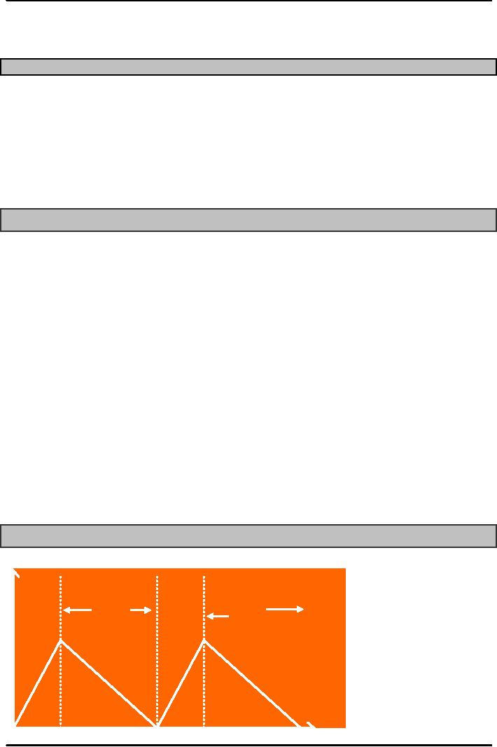
Economic Production Quantity (EPQ)

Production

Usage

& Usage Usage

& Usage

Inventory Level

152

Production and Operations Management MGT613

Economic Production Quantity (EPQ) Assumptions

Production done in batches or lots

Capacity to produce a part exceeds the part's usage or demand rate.

Assumptions of EPQ are similar to EOQ except orders are received incrementally during

production.

Economic Production Quantity Assumptions

Only one item is involved

Annual demand is known

Usage rate is constant

Usage occurs continuously

Production rate is constant

Lead time does not vary

No quantity discounts

Finer Points of Economic Production Quantity Model

The basic EOQ model assumes that each order is delivered at a single point in time.

If the firm is the producer and user, practical examples indicate that inventories are replenished

over time and not instantaneously.

If usage and production ( delivery) rates are equal, then there is no buildup of inventory.

Set up costs in a way our similar to ordering costs because they are independent of lot size.

The larger the run size, the fewer the number of runs needed and hence lower the annual setup.

The number of runs is D/Q and the annual setup cost is equal to the number of runs per year

times the cost per run ( D/Q)S.

Total Cost is

TC min= Carrying Cost+ Setup Cost

= ( I max/2)H+ (D/Q0)S

Where I max= Maximum Inventory

Economic Run Size

2DS

Q0 =

p-u

Economic Production Quantity Assumptions

Where p= production rate

U = usage rate

Economic Production Quantity Assumptions

The Run time ( the production phase of the cycle) is a function of the run size and production rate

Run time = Q0/p

The maximum and average inventory levels are

I max = Q0/p (p-u)

I average= I max/2

153

Production and Operations Management MGT613

Example (Economic Run Size)

Example for Economic Run Size

A firm in Sialkot produces 250,000 each world class footballs for both domestic and international

markets . It can make footballs at a rate of 2000 per day. The footballs are manufactured uniformly

over the whole year. Carrying cost is Rs. 100 per football and Setup cost for a production run is Rs.

2500. The manufacturing unit operates for 250 days per year.

Determine the

1. Optimal Run Size.

2. Minimum total annual cost for carrying and setup cost.

3. Cycle time for the Optimal Run Size.

4. Run time by using the formula

2DS

Q0 =

p-u

Solution

1. Optimal Run Size.

= Sq Root (2 X 250,000 X 2500/100 )( Sq Root (2 000 /2000-1000 ))

= 2500( sq.root2X2)=5000 footballs.

2. Minimum total annual cost for carrying and setup cost.

= Carrying Cost + Set up Cost

=( I max/2)H+ ( D/Q0)S

Where I max= Q0/p ((p-u))=5000/2000(1000)

=2500 footballs

Now TC= 2500/2 X 100 + (250,000/5000 )(2500)

=1250 X 100 + 125,000

=125,000+ 125,000

= Rs. 250,000.

3. Cycle time for the Optimal Run Size.

Q0/U=5000/1000= 5 days

4. Run time

Q0/p=5000/2000= 2.5 days

Quantity Discount : Price reductions for large orders are called Quantity Discounts.

Total Costs with Purchasing Cost

Annual

Purchasing

carrying

ordering

TC =

cost

TC =

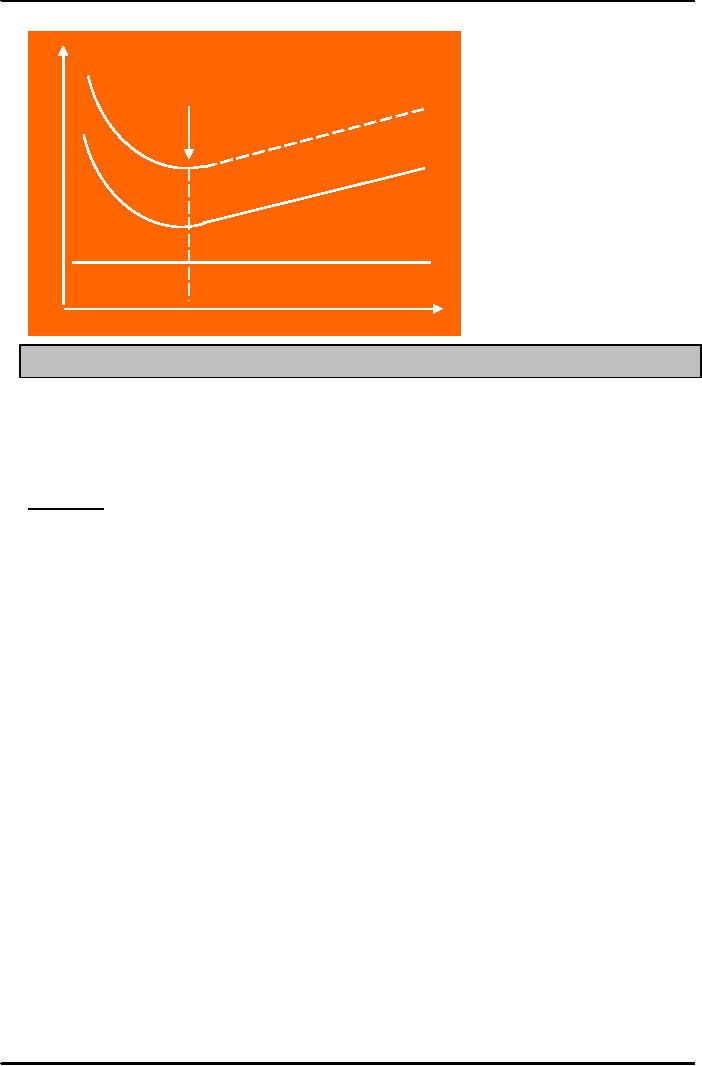
Total Costs with PD

154

Production and Operations Management MGT613

Adding Purchasing cost

TC with PD

doesn't change EOQ

TC without PD

Quantity

EOQ

Example for Optimal Order Quantity and Total Cost

The maintenance department of a large cardiology hospital in Islamabad uses about 1200 cases of

corrosion removal liquid, used for maintenance of hospital. Ordering costs are Rs 100, carrying cost

are Rs 20 per case, and the new price schedule indicates that orders of less than 50 cases will cost

Rs 1250 per case, 50 to 79 cases will cost Rs 1150 per case , 80 to 99 cases will cost Rs 1050 per

case and larger costs will be Rs 1000 per case.

Determine the Optimal Order Quantity and the Total Cost.

Given Data

D=1200 case.

S= Rs. 100 per case

H=Rs.20 per case

Range

Price

1 to 49

Rs 1250

50 to 79

Rs 1150

80 to 99

Rs 1050

100 or more

Rs 1000

Compute the Common EOQ=Sq Root (2DS/H)

= Sq Root (2 X 100 X 1200/20)

=Sq Root (12000)

=109.5=110 cases which would be brought at 1000 per order

The total Cost to Purchase 1200 cases per year would be

TC= Carrying Cost+ Order Cost+ Purchase Cost

=(Q/2)H+(D/Q0)S+PD

=(110/2)20+(1200/110)100+1200X 1000

=1100+1091+12000,000

=Rs. 1,202,191

155

Production and Operations Management MGT613

When to Reorder with EOQ Ordering

Reorder Point - When the quantity on hand of an item drops to this amount, the item is reordered.

Safety Stock - Stock that is held in excess of expected demand due to variable demand rate and/or

lead time.

Service Level - Probability that demand will not exceed supply during lead time.

Example for Reorder Point

An apartment complex in Quetta requires water for its home use.

Usage= 2 barrels a day

Lead time= 5 days

ROP= Usage X Lead Time

= 2 barrels a day X 7 = 14 barrels

Determinants of the Reorder Point

The rate of demand

The lead time

Stock out risk (safety stock)

Demand and/or lead time variability

Example

An owner of a Montessori equipment firm in Karachi, determined from historical records that

demand for wood required for Montessori equipment averages 25 tones per anum. His operations

management expertise allowed him to determine the demand during lead that could be described by

a normal distribution that has a mean of 25 tons and a standard deviation of 2.5 tons, with a stock

out risk not limited to 6 percent.

a. Appropriate value of Z? Please use the table given on the next page (9)

b. Safety stock level?

c. Reorder Point?

d. Expected weight of wood short for any order cycle, if he wants to maintain a service level of

80% Use the attached service level table. Please use the table given on page ( 10)

e. Annual Service Level, if service level =80

156

Production and Operations Management MGT613

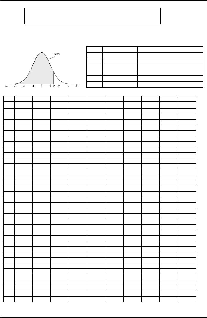
Area under the standardizes normal curve from -∞ to z

A(z) is the integral of the standardized normal distribution from ∞-to z (in other words, the area under the curve

to the left of z). It gives the probability of a normal random variable not being more than z standard deviations

above its mean. Values of z of particular importance:

A(z)

1.645

0.9500

Lower limit of right 5% tail

1.960

0.9750

Lower limit of right 2.5% tail

2.326

0.9900

Lower limit of right 1% tail

2.576

0.9950

Lower limit of right 0.5% tail

3.090

0.9990

Lower limit of right 0.1% tail

3.291

0.9995

Lower limit of right 0.05% tail

Cumulative Standardized Normal Distribution

0.00

0.01

0.02

0.03

0.04

0.05

0.06

0.07

0.08

0.09

0.0

0.5000

0.5040

0.5080

0.5120

0.5160

0.5199

0.5239

0.5279

0.5319

0.5359

0.1

0.5398

0.5438

0.5478

0.5517

0.5557

0.5596

0.5636

0.5675

0.5714

0.5753

0.2

0.5793

0.5832

0.5871

0.5910

0.5948

0.5987

0.6026

0.6064

0.6103

0.6141

0.3

0.6179

0.6217

0.6255

0.6293

0.6331

0.6368

0.6406

0.6443

0.6480

0.6517

0.4

0.6554

0.6591

0.6628

0.6664

0.6700

0.6736

0.6772

0.6808

0.6844

0.6879

0.5

0.6915

0.6950

0.6985

0.7019

0.7054

0.7088

0.7123

0.7157

0.7190

0.7224

0.6

0.7257

0.7291

0.7324

0.7357

0.7389

0.7422

0.7454

0.7486

0.7517

0.7549

0.7

0.7580

0.7611

0.7642

0.7673

0.7704

0.7734

0.7764

0.7794

0.7823

0.7852

0.8

0.7881

0.7910

0.7939

0.7967

0.7995

0.8023

0.8051

0.8078

0.8106

0.8133

0.9

0.8159

0.8186

0.8212

0.8238

0.8264

0.8289

0.8315

0.8340

0.8365

0.8389

1.0

0.8413

0.8438

0.8461

0.8485

0.8508

0.8531

0.8554

0.8577

0.8599

0.8621

1.1

0.8643

0.8665

0.8686

0.8708

0.8729

0.8749

0.8770

0.8790

0.8810

0.8830

1.2

0.8849

0.8869

0.8888

0.8907

0.8925

0.8944

0.8962

0.8980

0.8997

0.9015

1.3

0.9032

0.9049

0.9066

0.9082

0.9099

0.9115

0.9131

0.9147

0.9162

0.9177

1.4

0.9192

0.9207

0.9222

0.9236

0.9251

0.9265

0.9279

0.9292

0.9306

0.9319

1.5

0.9332

0.9345

0.9357

0.9370

0.9382

0.9394

0.9406

0.9418

0.9429

0.9441

1.6

0.9452

0.9463

0.9474

0.9484

0.9495

0.9505

0.9515

0.9525

0.9535

0.9545

1.7

0.9554

0.9564

0.9573

0.9582

0.9591

0.9599

0.9608

0.9616

0.9625

0.9633

1.8

0.9641

0.9649

0.9656

0.9664

0.9671

0.9678

0.9686

0.9693

0.9699

0.9706

1.9

0.9713

0.9719

0.9726

0.9732

0.9738

0.9744

0.9750

0.9756

0.9761

0.9767

2.0

0.9772

0.9778

0.9783

0.9788

0.9793

0.9798

0.9803

0.9808

0.9812

0.9817

2.1

0.9821

0.9826

0.9830

0.9834

0.9838

0.9842

0.9846

0.9850

0.9854

0.9857

2.2

0.9861

0.9864

0.9868

0.9871

0.9875

0.9878

0.9881

0.9884

0.9887

0.9890

2.3

0.9893

0.9896

0.9898

0.9901

0.9904

0.9906

0.9909

0.9911

0.9913

0.9916

2.4

0.9918

0.9920

0.9922

0.9925

0.9927

0.9929

0.9931

0.9932

0.9934

0.9936

2.5

0.9938

0.9940

0.9941

0.9943

0.9945

0.9946

0.9948

0.9949

0.9951

0.9952

2.6

0.9953

0.9955

0.9956

0.9957

0.9959

0.9960

0.9961

0.9962

0.9963

0.9964

2.7

0.9965

0.9966

0.9967

0.9968

0.9969

0.9970

0.9971

0.9972

0.9973

0.9974

2.8

0.9974

0.9975

0.9976

0.9977

0.9978

0.9979

0.9980

0.9981

2.9

0.9981

0.9982

0.9983

0.9984

0.9985

0.9986

3.0

0.9987

0.9988

0.9989

0.9990

3.1

0.9990

0.9991

0.9992

0.9993

3.2

0.9993

0.9994

0.9995

3.3

0.9995

0.9996

0.9997

3.4

0.9997

0.9998

3.5

0.9998

157

Production and Operations Management MGT613

158

Production and Operations Management MGT613

SOLUTION

a. Expected Lead Time Demand= 25 tonnes, also σdLT= 2.5 tonnes, Risk= 6%. Using the given

table values, 1-0.06=.9400 therefore + Z=1.1.55

b. The safety stock = ZσdLT= 1.55 x 2.50 tonnes= 3.875 tonnes

c. Reorder Point =

Expected Lead Time Demand + Safety Stock

25 tonnes + 3.875=28.875 tonnes

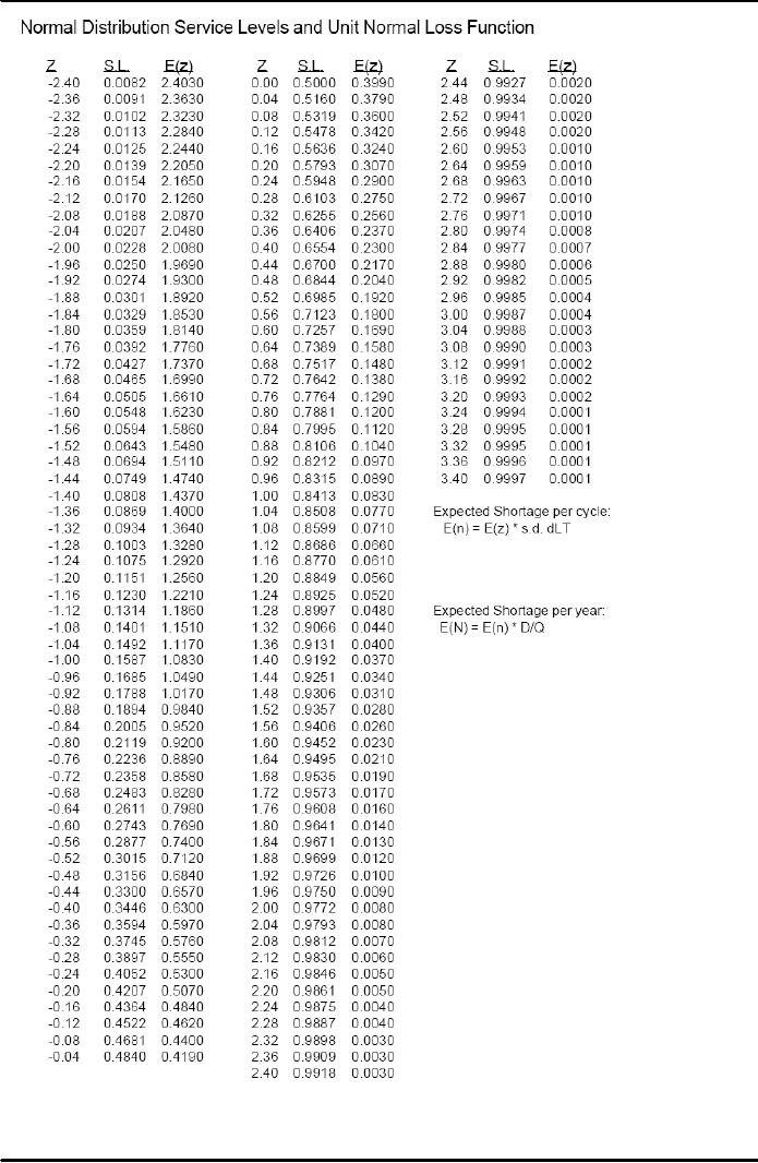
d. From the Service Level Table, Lead time Service Level z=0.8 therefore E(z)=0.7881,using the

formula E(n)=E(z) X σdLT

Now Since σ dLT= 2.5 tonnes

Therefore E(n)=0.7881(2.50)=39.41 tonnes= 1.97025 tonnes

e. SL annual= 1-E(z) σdLT/Q

Now Since Q= 25 tonnes, E(z)=

We can calculate the Annual Service Level by substituting values in the formula above

SL annual= 1-0.7881(50)/1000=1-39.405/1000=1-0.03941=0.961

Fixed-Order-Interval Model

Orders are placed at fixed time intervals.

Order quantity for next interval?

Suppliers might encourage fixed intervals.

May require only periodic checks of inventory levels.

Risk of stock out.

Summary

In this lecture we studied various important concepts relating to Inventory Management. Most

importantly we learnt how to make use of statistical tables to calculate lead points and service levels.

This lecture forms the basis for Supply Chain Management and Just In Time Production Systems.

159

Table of Contents: