 |
GEOMETRIC MEAN:MEAN DEVIATION FOR GROUPED DATA |
| << GEOMETRIC MEAN:Number of Pupils, QUARTILE DEVIATION: |
| COUNTING RULES:RULE OF PERMUTATION, RULE OF COMBINATION >> |
MTH001
Elementary Mathematics
LECTURE #
28:
·
Mean
Deviation
·
Standard
Deviation and
Variance
·
Coefficient
of variation
First,
we will discuss it for the
case of raw data, and
then we will go on to the
case of a
frequency
distribution. The first
thing to note is that,
whereas the range as well as
the
quartile
deviation are two such
measures of dispersion which
are NOT based on all
the
values,
the mean deviation and
the standard deviation are
two such measures of
dispersion
that
involve each and every
data-value in their
computation.
You
must have noted that
the range was measuring
the dispersion of the
data-set
around
the mid-range, whereas the
quartile deviation was
measuring the dispersion of
the
data-set
around the median.
How
are we to decide upon the
amount of dispersion round
the arithmetic mean?
It
would
seem reasonable to compute
the DISTANCE of each
observed value in the
series
from
the arithmetic mean of the
series.
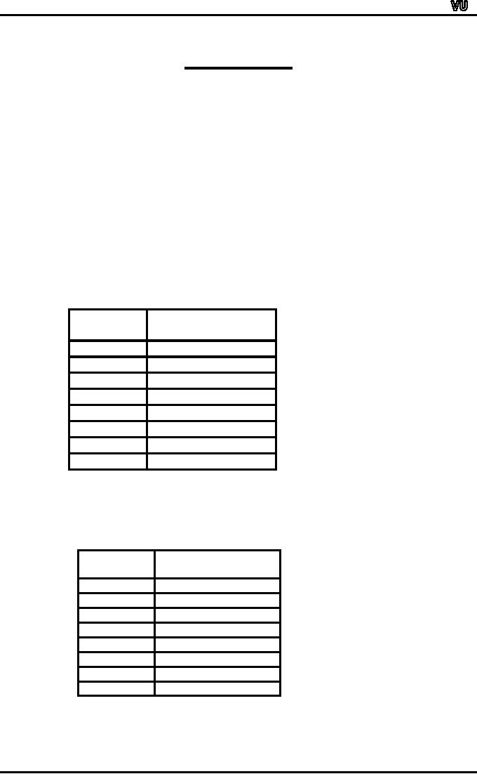
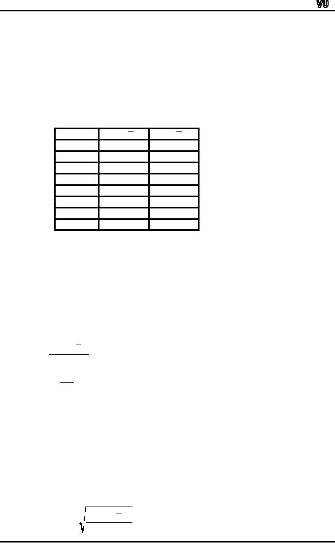
Let
us do this for a simple
data-set shown below:
The
Number of Fatalities in Motorway
Accidents in one
Week:
Number
of fatalities
Day
X
Sunday
4
Monday
6
Tuesday
2
Wednesday
0
Thursday
3
Friday
5
Saturday
8
Total
28
Let
us do this for a simple
data-set shown below:
The
Number of Fatalities in Motorway
Accidents in one
Week:
Number
of fatalities
Day
X
Sunday
4
Monday
6
Tuesday
2
Wednesday
0
Thursday
3
Friday
5
Saturday
8
Total
28
Page
195
MTH001
Elementary Mathematics
The
arithmetic mean number of
fatalities per day is
∑
X
=
28
=
4
X=
n
7
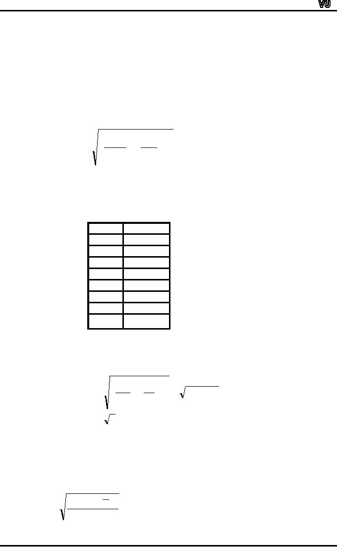
In
order to determine the
distances of the data-values
from the mean, we subtract
our value
of
the arithmetic mean from
each daily figure, and
this gives us the deviations
that occur in
the
third column of the table
below:
Number
of fatalities
X-X
Day
X
Sunday
4
0
Monday
6
+2
Tuesday
2
2
Wednesday
0
4
Thursday
3
1
Friday
5
+1
Saturday
8
+4
TOTAL
28
0
The
deviations are negative when
the daily figure is less
than the mean (4 accidents)
and
positive
when the figure is higher
than the mean.
It
does seem, however, that
our efforts for computing
the dispersion of this data
set have
been
in vain, for we find that
the total amount of
dispersion obtained by summing
the
(x
⎯x)
column comes out to be zero!
In fact, this should be no
surprise, for it is a
basic
property
of the arithmetic mean
that:The sum of the
deviations of the values
from the mean
is
zero.
The
question arises:
How
will we measure the
dispersion that is actually
present in our
data-set?
Our
problem might at first sight
seem irresolvable, for by
this criterion it appears
that no
series
has any dispersion. Yet we
know that this is absolutely
incorrect, and we must think
of
some
other way of handling this
situation. Surely, we might
look at the numerical
difference
between
the mean and the
daily fatality figures
without considering whether
these are
positive
or negative.
Let
us denote these absolute
differences by `modulus of d' or `mod
d'.
This
is evident from the third
column of the table
below:
X
⎯X =
d
X
|d|
4
0
0
6
2
2
2
2
2
0
4
4
3
1
1
5
1
1
8
4
4
Total
14
Page
196
MTH001
Elementary Mathematics
By
ignoring the sign of the
deviations we have achieved a
non-zero sum in our
second
column.
Averaging these absolute
differences, we obtain a measure of
dispersion known as
the
mean deviation.
In
other words, the mean
deviation is given by the
formula:
MEAN
DEVIATION:
∑
|
di |
M.D.
=
n
As
we are averaging the
absolute deviations of the
observations from their
mean, therefore
the
complete name of this
measure is mean absolute
deviation --- but generally
we just say
"mean
deviation". Applying this
formula in our example, we
find that:
The
mean deviation of the number
of fatalities is
14
M.D.
=
=
2.
7
The
formula that we have just
considered is valid in the
case of raw data. In case of
grouped
data
i.e. a frequency distribution,
the formula becomes
MEAN
DEVIATION FOR GROUPED
DATA:
∑
fi x i
-
x
∑
fi di
M.D.
=
=
n
n
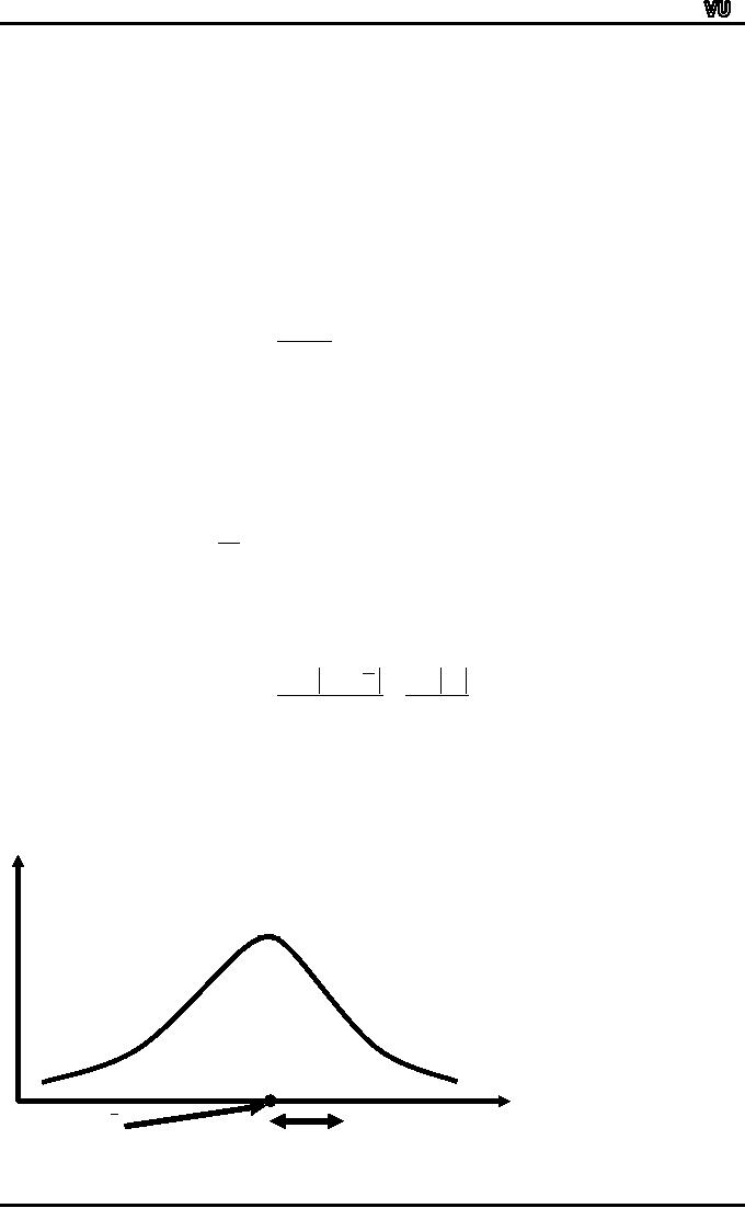
As
far as the graphical
representation of the mean
deviation is concerned, it can be
depicted
by
a
horizontal
line
segment
drawn
below
the
X-axis
on the graph of the
frequency distribution, as shown
below:
f
X
X
Mean
Deviation
Page
197
MTH001
Elementary Mathematics
The
approach which we have
adopted in the concept of
the mean deviation is both
quick
and
simple. But the problem is
that we introduce a kind of
artificiality in its calculation
by
ignoring
the algebraic signs of the
deviations.
In
problems involving descriptions
and comparisons alone, the
mean deviation can
validly
be
applied; but because the
negative signs have been
discarded, further
theoretical
development
or application of the concept is
impossible.
Mean
deviation is an absolute measure of
dispersion. Its relative
measure, known as
the
co-efficient of mean deviation, is
obtained by dividing the
mean deviation by the
average
used
in the calculation of deviations
i.e. the arithmetic mean.
Thus
Co-efficient
of M.D:
Sometimes,
the mean deviation is
co.D.uted
by averaging the absolute
deviations of the
Mmp
data-values
from the median i.e.
=
Mean
∑
x-~
x
Mean
deviation =
n
And
when will we have a
situation when we will be
using the median instead of
the
mean?As
discussed earlier, the
median will be more
appropriate than the mean in
those
cases
where our data-set contains
a few very high or very
low values.In such a
situation, the
coefficient
of mean deviation is given
by:
Co-efficient
of M.D:
M.D.
=
Median
Let
us now consider the
standard
deviation ---
that statistic which is the
most important and
the
most widely used measure of
dispersion.
The
point that made earlier
that from the mathematical
point of view, it is not
very preferable
to
take the absolute values of
the deviations, This
problem is overcome by computing
the
standard
deviation.
In
order to compute the
standard deviation, rather
than taking the absolute
values of the
deviations,
we square the
deviations.
Averaging
these squared deviations, we
obtain a statistic that is
known as the
variance.
Variance
∑
(x
-
x )
2
=
n
Let
us compute this quantity for
the data of the above
example.
Our
X-values were:
X
4
6
2
0
3
Page
5
198
8
MTH001
Elementary Mathematics
Taking
the deviations of the
X-values from their mean,
and then squaring these
deviations,
we
obtain:
(x -
x )
(
x -
x )2
X
4
0
0
6
+2
4
2
2
4
0
4
16
3
1
1
5
+1
1
8
+4
16
42
Obviously,
both ( 2)2 and (2)2
equal 4, both ( 4)2 and
(4)2 equal 16, and
both ( 1)2 and
(1)2
= 1.
Hence
∑(x
⎯x)2
= 42 is now positive, and
this positive value has
been achieved
without
`bending' the rules of
mathematics. Averaging these
squared deviations,
the
variance
is given by:
Variance:
∑
(x
-
x
)
2
=
n
42
=
=6
7
The
variance is frequently employed in
statistical work, but it
should be noted that the
figure
achieved
is in `squared' units of
measurement.
In
the example that we have
just considered, the
variance has come out to be
"6 squared
fatalities",
which does not seem to
make much sense!
In
order to obtain an answer
which is in the original
unit of measurement, we take
the
positive
square root of the variance.
The result is known as the
standard deviation.
STANDARD
DEVIATION:
∑
(x
-
x )
2
S=
n
Page
199
MTH001
Elementary Mathematics
Hence,
in this example, our
standard deviation has come
out to be 2.45
fatalities.
In
computing the standard
deviation (or variance) it
can be tedious to first
ascertain
the
arithmetic mean of a series,
then subtract it from each
value of the variable in the
series,
and
finally to square each
deviation and then
sum.
It
is very much more
straight-forward to use the
short cut formula given
below:
SHORT
CUT FORMULA FOR THE
STANDARD DEVIATION:
⎧
∑ x
2 ⎛
∑ x
⎞2
⎫
⎪
⎪
S=
⎨
-⎜
⎟ ⎬
⎪ n
⎝ n ⎠ ⎪
⎩
⎭
In
order to apply the short
cut formula, we require only
the aggregate of the series
(∑x)
and
the
aggregate of the squares of
the individual values in the
series (∑x2).
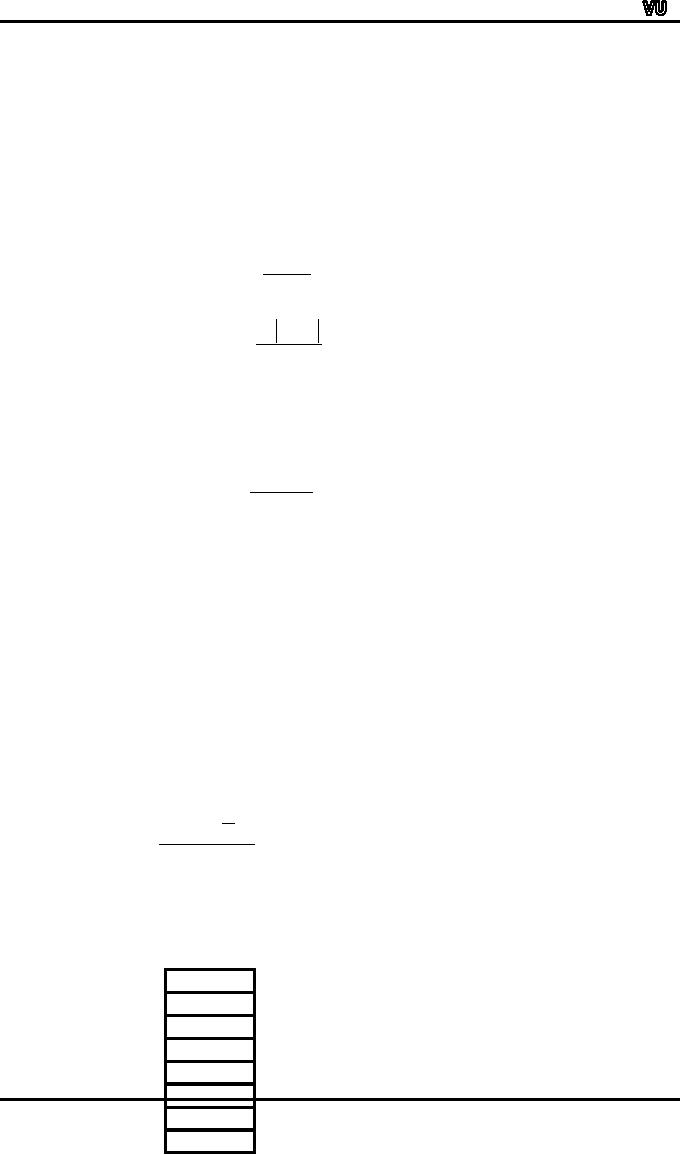
In
other words, only two
columns of figures are
called for. The number of
individual
calculations
is also considerably reduced, as
seen below:
X2
X
4
16
6
36
2
4
0
0
3
9
5
25
8
64
Total
28
154
Therefore
⎧154
⎛
28
⎞2
⎫
⎪
⎪
(22
-
16)
S=
⎨
-⎜
⎟ ⎬ =
⎪ 7 ⎝7⎠ ⎪
⎩
⎭
=
6
=
2.45
fatalities
The
formulae that we have just
discussed are valid in case
of raw data. In case of
grouped
data
i.e. a frequency distribution,
each squared deviation round
the mean must be
multiplied
by
the appropriate frequency
figure i.e.
STANDARD
DEVIATION IN CASE OF GROUPED
DATA:
∑
f
(x
-
x )
2
S=
n
Page
200
MTH001
Elementary Mathematics
And
the short cut formula in
case of a frequency distribution
is:
SHORT
CUT FORMULA OF THE STANDARD
DEVIATION IN CASE OF
GROUPED
DATA:
⎧
fx
2 ⎛
fx
⎞
⎫
⎪∑
∑
⎟ ⎪
2
-⎜
S=
⎨
⎜
n
⎟ ⎬
n
⎪
⎠ ⎪
⎝
⎩
⎭
Which
is again preferred from the
computational standpoint?
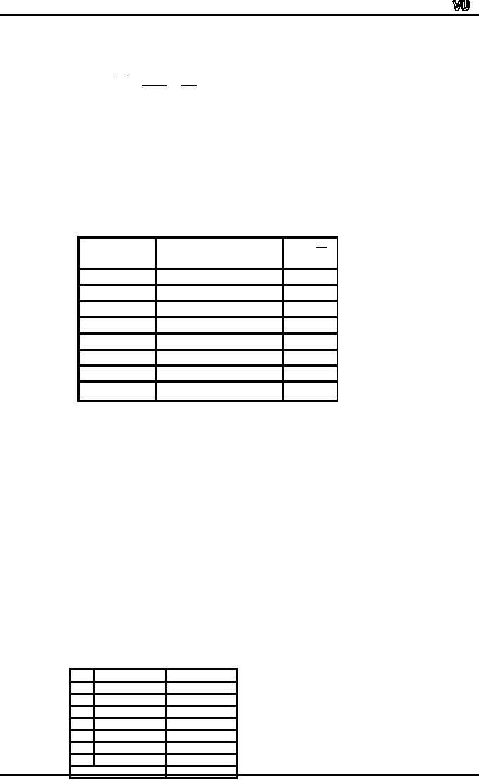
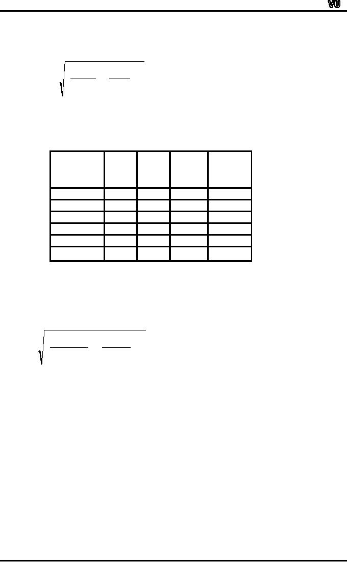
For
example, the standard
deviation life of a batch of
electric light bulbs would
be calculated
as
follows:
EXAMPLE:
Life
(in
No.
of
Mid-
fx2
Hundreds
Bulbs
point
fx
of
Hours)
f
x
05
4
2.5
10.0
25.0
5
10
9
7.5
67.5
506.25
10
20
38
15.0
570.0
8550.0
20
40
33
30.0
990.0
29700.0
40
and over
16
50.0
800.0
40000.0
100
2437.5
78781.25
Therefore,
standard
deviation:
⎧
78781.25
⎛
2437.5
⎞2
⎫
⎪
⎪
S=
⎨
-⎜
⎟ ⎬
⎪
100
⎝
100
⎠
⎪
⎩
⎭
=13.9hundredhours
=
1390 hours
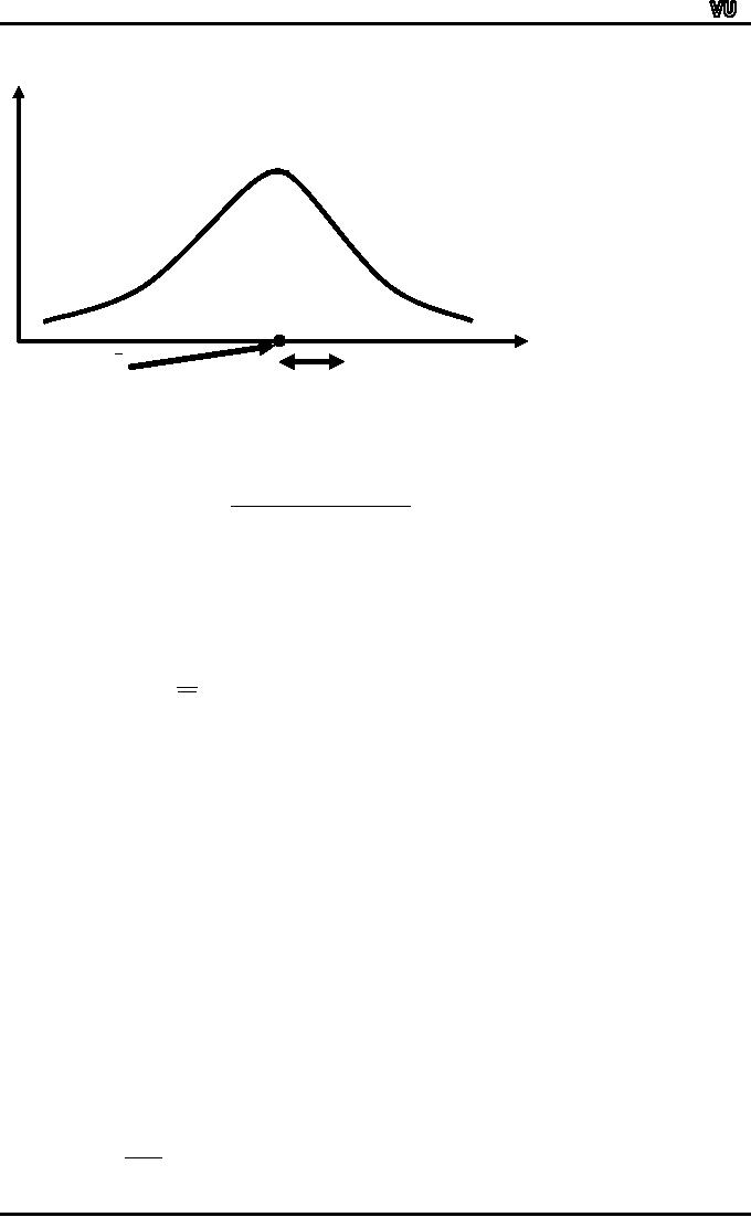
As
far as the graphical
representation of the standard
deviation is concerned, a
horizontal
line
segment is drawn below the
X-axis on the graph of the
frequency distribution ---
just as
in
the case of the mean
deviation.
Page
201
MTH001
Elementary Mathematics
f
X
X
Standard
deviation
The
standard deviation is an absolute
measure of dispersion. Its
relative measure
called
coefficient
of standard deviation is defined
as:
Coefficient
of S.D:
S
tan dard Deviation
=
Mean
And,
multiplying this quantity by
100, we obtain a very
important and well-known
measure
called
the coefficient of
variation.
Coefficient
of Variation:
S
C.V.
=
×100
X
As
mentioned earlier, the
standard deviation is expressed in
absolute terms and is given
in
the
same unit of measurement as
the variable itself.
There
are occasions, however, when
this absolute measure of
dispersion is inadequate
and
a
relative form becomes
preferable.
For
example, if a comparison between
the variability of distributions
with different
variables
is required, or when we need to
compare the dispersion of
distributions with
the
same
variable but with very
different arithmetic
means.
To
illustrate the usefulness of
the coefficient of variation,
let us consider the
following
two
examples:
EXAMPLE-1
Suppose
that, in a particular year,
the mean weekly earnings of
skilled factory workers
in
one
particular country were $
19.50 with a standard
deviation of $ 4, while for
its neighboring
country
the figures were Rs. 75
and Rs. 28
respectively.
From
these figures, it is not
immediately apparent which
country has the
GREATER
VARIABILITY
in earnings.
The
coefficient of variation quickly
provides the answer:
COEFFICIENT
OF VARIATION
For
country No. 1:
4
×
100
=
20.5
per
cent,
19.5
Page
202

MTH001
Elementary Mathematics
And
for country No. 2:
28
×100
=
37.3
per cent.
75
From
these calculations, it is immediately
obvious that the spread of
earnings in country
No.
2
is greater than that in
country No. 1, and the
reasons for this could
then be sought.
EXAMPLE-2:
The
crop yield from 20 acre
plots of wheat-land cultivated by
ordinary methods averages
35
bushels
with a standard deviation of 10
bushels. The yield from
similar land treated with
a
new
fertilizer averages 58 bushels,
also with a standard
deviation of 10 bushels. At
first
glance,
the yield variability may
seem to be the same, but in
fact it has improved
(i.e.
decreased)
in view of the higher
average to which it
relates.
Again,
the coefficient of variation
shows this very
clearly:
Coefficient
of Variation:
Untreated
land:
10
×
100
=
28.57
per cent
35
Treated
land:
10
×
100
=
17.24
per cent
58
The
coefficient of variation for
the untreated land has
come out to be 28.57
percent,
whereas
the coefficient of variation
for the treated land is
only 17.24 percent.
Page
203
Table of Contents:
- Recommended Books:Set of Integers, SYMBOLIC REPRESENTATION
- Truth Tables for:DE MORGANS LAWS, TAUTOLOGY
- APPLYING LAWS OF LOGIC:TRANSLATING ENGLISH SENTENCES TO SYMBOLS
- BICONDITIONAL:LOGICAL EQUIVALENCE INVOLVING BICONDITIONAL
- BICONDITIONAL:ARGUMENT, VALID AND INVALID ARGUMENT
- BICONDITIONAL:TABULAR FORM, SUBSET, EQUAL SETS
- BICONDITIONAL:UNION, VENN DIAGRAM FOR UNION
- ORDERED PAIR:BINARY RELATION, BINARY RELATION
- REFLEXIVE RELATION:SYMMETRIC RELATION, TRANSITIVE RELATION
- REFLEXIVE RELATION:IRREFLEXIVE RELATION, ANTISYMMETRIC RELATION
- RELATIONS AND FUNCTIONS:FUNCTIONS AND NONFUNCTIONS
- INJECTIVE FUNCTION or ONE-TO-ONE FUNCTION:FUNCTION NOT ONTO
- SEQUENCE:ARITHMETIC SEQUENCE, GEOMETRIC SEQUENCE:
- SERIES:SUMMATION NOTATION, COMPUTING SUMMATIONS:
- Applications of Basic Mathematics Part 1:BASIC ARITHMETIC OPERATIONS
- Applications of Basic Mathematics Part 4:PERCENTAGE CHANGE
- Applications of Basic Mathematics Part 5:DECREASE IN RATE
- Applications of Basic Mathematics:NOTATIONS, ACCUMULATED VALUE
- Matrix and its dimension Types of matrix:TYPICAL APPLICATIONS
- MATRICES:Matrix Representation, ADDITION AND SUBTRACTION OF MATRICES
- RATIO AND PROPORTION MERCHANDISING:Punch recipe, PROPORTION
- WHAT IS STATISTICS?:CHARACTERISTICS OF THE SCIENCE OF STATISTICS
- WHAT IS STATISTICS?:COMPONENT BAR CHAR, MULTIPLE BAR CHART
- WHAT IS STATISTICS?:DESIRABLE PROPERTIES OF THE MODE, THE ARITHMETIC MEAN
- Median in Case of a Frequency Distribution of a Continuous Variable
- GEOMETRIC MEAN:HARMONIC MEAN, MID-QUARTILE RANGE
- GEOMETRIC MEAN:Number of Pupils, QUARTILE DEVIATION:
- GEOMETRIC MEAN:MEAN DEVIATION FOR GROUPED DATA
- COUNTING RULES:RULE OF PERMUTATION, RULE OF COMBINATION
- Definitions of Probability:MUTUALLY EXCLUSIVE EVENTS, Venn Diagram
- THE RELATIVE FREQUENCY DEFINITION OF PROBABILITY:ADDITION LAW
- THE RELATIVE FREQUENCY DEFINITION OF PROBABILITY:INDEPENDENT EVENTS