Elasticities of supply and demand:The Demand for Gasoline

<< Changes in Market Equilibrium:Market for College Education

Consumer Behavior:Consumer Preferences, Indifference curves >>

Microeconomics ECO402

LESSON 5

Elasticities of supply and demand

Other Demand Elasticities

Income elasticity of demand measures the percentage change in quantity

demanded resulting from a one percent change in income.

The income elasticity of demand is:

ΔQ/Q

I ΔQ

EI =

ΔI/I

Q ΔI

Income Elasticity of Demand

Quantity

for:

Income Elasticity

Demanded

Normal goods

less than 1 (but

greater than 0)

Superior goods

Normal goods

Inferior goods

Negative

Income

Elasticity

Inferior

greater than 1

goods

superior

goods

Money

Income

Other Demand Elasticities

Cross elasticity of demand measures the percentage change in the quantity

demanded of one good that results from a one percent change in the price of

another good.

For example consider the substitute goods, butter and margarine.

The cross elasticity of demand is:

ΔQb/Qb Pm ΔQb

EQbPm =

ΔPm/Pm Qb ΔPm

Cross elasticity for substitutes is positive

Cross elasticity for complements is negative

♦ Price elasticity of supply

measures the percentage change in quantity supplied resulting from a 1

percent change in price.

The elasticity is usually positive because price and quantity supplied are directly

related.

We can refer to elasticity of supply with respect to interest rates, wage rates,

and the cost of raw materials.

Price ($)

Quantity Demanded

Quantity Supplied

100

120

Microeconomics ECO402

Recall

ΔQ/Q

P ΔQ

EP =

ΔP/P

Q ΔP

Elasticity of demand when price is $80 is

Ep = 80/20 x -2/20 = -0.40

Elasticity of demand when price is $100 is

Ep = 100/18 x -2/20 = -0.56

Elasticity of supply when price is $80 is

Ep = 80/16 x 2/20 = 0.50

Elasticity of supply when price is $100 is

Ep = 100/18 x 2/20 = 0.56

The Market for Wheat

1981 Supply Curve for Wheat

QS = 1,800 + 240P

1981 Demand Curve for Wheat

QD = 3,550 - 266P

Equilibrium: Q S = Q D

1, 800 + 240P = 3, 550 - 266P

506P = 1, 750

P = 3.46 / bushel

Q = 1, 800 + (240)(3.46) = 2, 630 million bushels

P ΔQD

3.46

EP =

(-2.66) = -.035 Inelastic

Q ΔP

2, 630

P ΔQS

3.46

EP =

(2.40) = .032 Inelastic

Q ΔP

2, 630

Assume the price of wheat is $4.00/bushel

QD = 3, 550 - (266)(4.00) = 2, 486

4.00

QP =

(-266) = -0.43

2, 486

Supply (Qs)

Demand (Qd)

Equilibrium Price

Qs = Qd

1981

1800 + 240P

3550 266P

1800 + 240P = 3550 266P

506P = 1750

P1981 = $3.46 / bushel

1998

1944 + 207P

3244 283P

1944 +207P = 3244 283P

P1998 = $2.65 / bushel

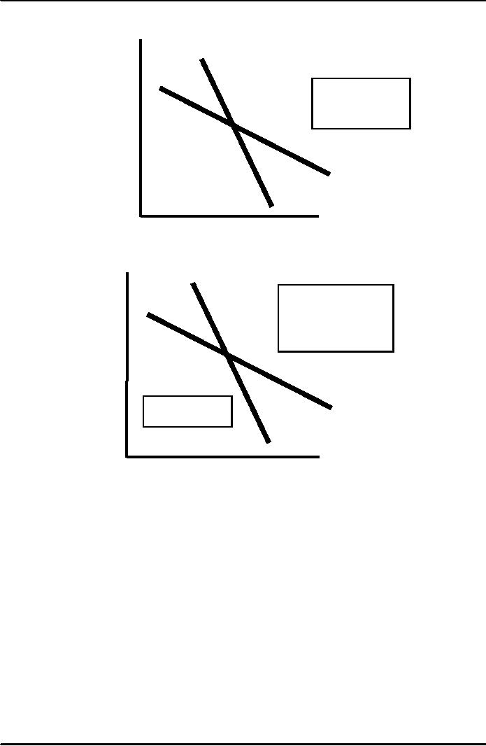
Short-Run Versus Long-Run Elasticities

Price elasticity of demand varies with the amount of time consumers have to respond

to a price.

Most goods and services:

Short-run elasticity is less than long-run elasticity. (e.g. gasoline, Drs.)

Other Goods (durables):

Short-run elasticity is greater than long-run elasticity (e.g. automobiles)

Microeconomics ECO402

Gasoline: Short-Run and Long-Run Demand Curves

DSR

Price

People tend to

drive smaller and

more fuel efficient

cars in the long-run

Gasoline

DLR

Quantity

Automobiles: Short-Run and Long-Run Demand Curves

DLR

Price

People may put off

immediate consumption,

but eventually older cars

must be replaced.

Automobiles

DSR

Quantity

Income elasticity also varies with the amount of time consumers have to respond to an

income change.

Most goods and services:

Income elasticity is greater in the long-run than in the short run.

Higher incomes may be converted into bigger cars so the income

elasticity of demand for gasoline increases with time.

Other Goods (durables):

Income elasticity is less in the long-run than in the short-run.

Originally, consumers will want to hold more cars.

Later, purchases will only to be to replace old cars.

Gasoline and Automobiles are complementary goods.

Gasoline

The long-run price and income elasticities are larger than the short-run

elasticities.

Automobiles

The long-run price and income elasticities are smaller than the short-run

elasticities.

Microeconomics ECO402

The Demand for Gasoline

Years Following price or income change

Elasticity

Price

-0.11

-0.22

-0.32

-0.49

-0.82

-1.17

Income

0.07

0.13

0.20

0.32

0.54

0.78

The Demand for Automobiles

Years Following price or income change

Elasticity

Price

-1.20

-0.93

-0.75

-0.55

-0.42

-0.40

Income

3.00

2.33

1.88

1.38

1.02

1.00

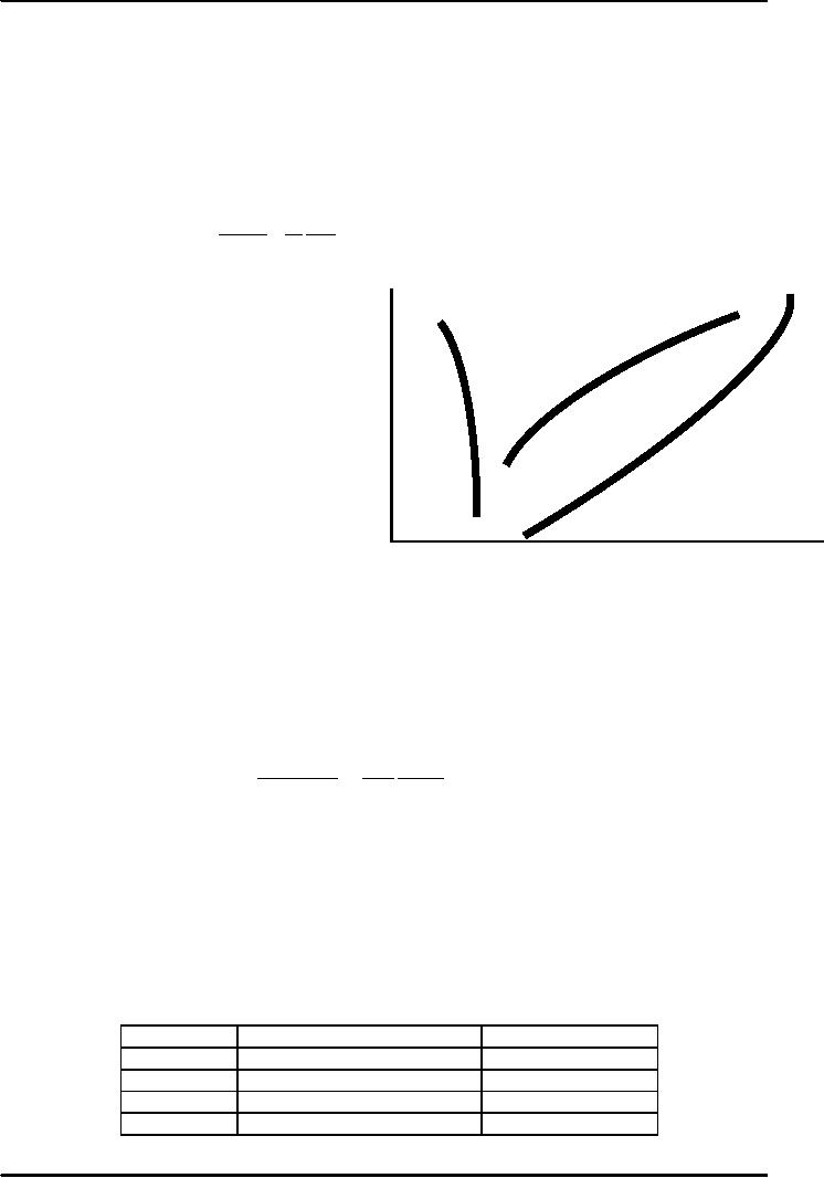
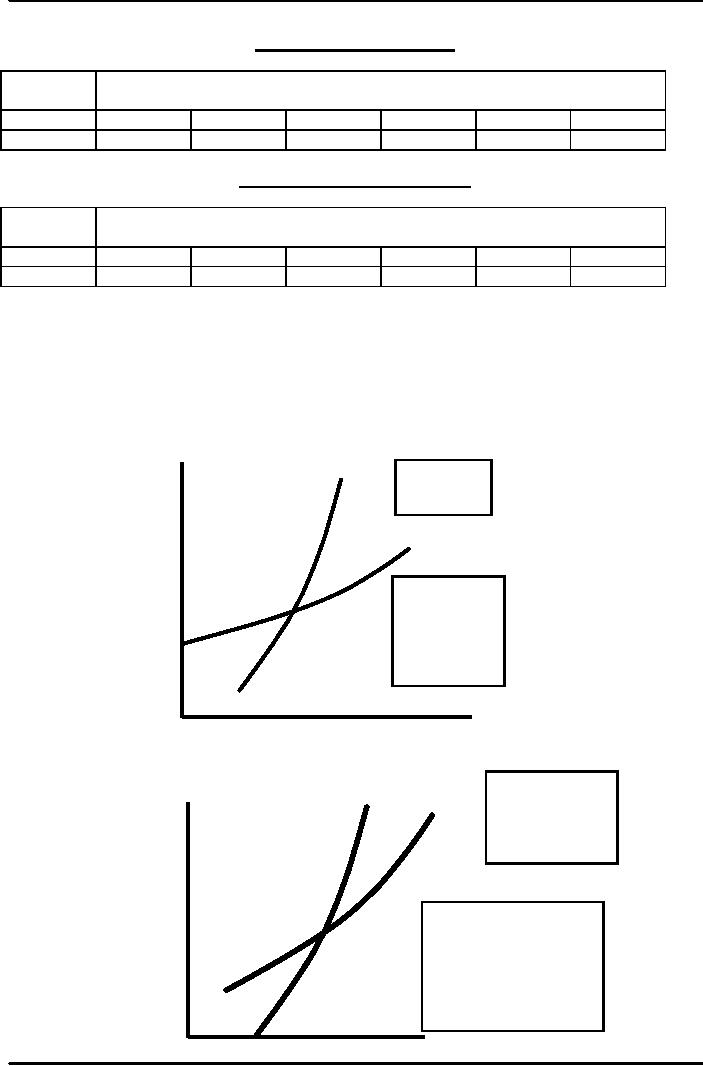
Supply

Most goods and services:

· Long-run price elasticity of supply is greater than short-run price

elasticity of supply.

Other Goods (durables, recyclables):

· Long-run price elasticity of supply is less than short-run price elasticity of

supply

SSR

Price

Primary Copper:

Short-Run and

Long-Run

Supply Curves

SLR

Due to limited

capacity, firms are

limited by output

constraints in the

short-run. In the

long-run, they can

expand.

Quantity

Secondary

Copper: Short-Run

Pric

and

Long-Run Supply

Curves

Price increases

provide an incentive

to convert scrap

copper into new supply.

In the long-run, this

stock of scrap copper

begins to fall.

Quantity

Microeconomics ECO402

Supply of Copper

Price Elasticity of:

Short Run

Long run

Primary Supply

0.20

1.60

Secondary Supply

0.43

0.31

Total Supply

0.25

1.50

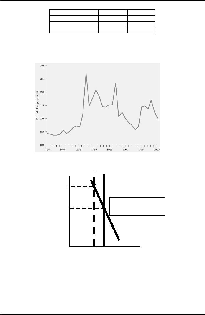
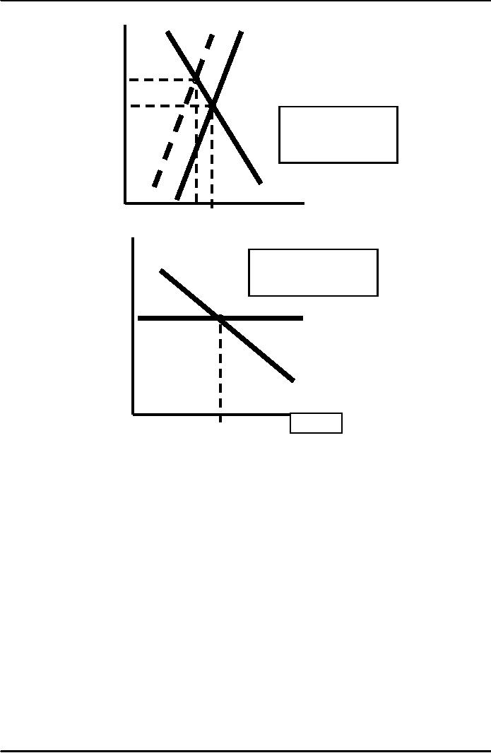
Weather in Brazil and the price of Coffee in New York

Elasticity explains why coffee prices are very volatile.

Due to the differences in supply elasticity in the long-run and short run.

A freeze or drought

Price

decreases the

Coffee

supply

Short-Run

1) Supply is completely inelastic

2) Demand is relatively inelastic

3) Very large change in price

Quantity

Microeconomics ECO402

Price

Intermediate-Run

1) Supply and demand are

more elastic

2) Price falls back to P2.

3) Quantity falls to Q2

Quantity

Q2 Q0

Price

Long-Run

1 Supply is extremely elastic.

2) Price falls back to P0.

3) Quantity increase to Q0.

Quantity

Table of Contents: