 |
Lecture#
31
Supervised
Vs. Unsupervised
Learning
In the
previous lecture we discussed
briefly DM concepts. Now we
look with some
greater
details,
two main DM methods
supervised and unsupervised learning.
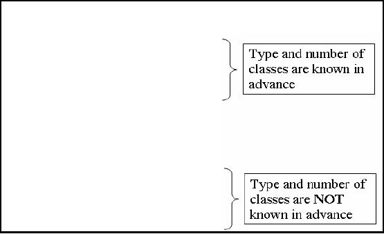
Supervised learning is
when you
are performing DM the supporting
information that helps in
the DM process is
also
available. What
could be that information? You
may know your data
that how many groups
or
classes
your data set contains.
What are the properties of
these classes or clusters?
When we will
talk about
unsupervised learning you will not have
such known or a priori knowledge. In
other
words you can
not give such factors as
input to the DM technique
which can facilitate your
DM
process. So
wherever the user gives
some input that is
supervised else that is
unsupervised
learning.
Data
Structures in Data Mining
§
Data
matrix
§ Table or
database
§ n
records
and m
attributes,
§ n
>>
m
§
Similarity
matrix
§ Symmetric
square
matrix
§ n
x
n
or
m
x
m
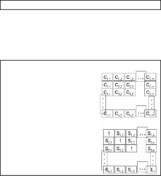
Figure
31.1: Data Structures in
data mining
First of all we
will talk about data
structures in DM. What does
DS mean here? You can
consider
it as pure
data structure but we specifically
mean how you store
your data. Figure 31.1
shows
two
metrics data matrix and the
similarity matrix. Data matrix means
the table or database
used
as the
input to the DM algorithm.
What will be the dimensions
or size of that table normally?
The
size of
records (rows) is much
greater th an the number of columns.
The attributes may be 10,
15
or 25 but the
number of rows far exceeds the number of
columns e.g. a customer
table may have
20-25 attributes
but the total records
may be in millions. As I said previously
that the mobile
users in Pa
kistan are about 10 million.
If a company even has 1/3 of
the customers then 3.3
lakh
customer
records in the customer
table. Thus greater number of rows than
columns and there
will
be indices
i
and
j
in
the table and you can pick
the particular contents o f a cell by
considering the
intersection of
the two indices.
256
The
second matrix in the Figure 31.1 is
called the similarity matrix.
Lets talk about its
brief
background.
Similarity or dissimilarity matrix is the
measure the similarity or
dissimilarity
obtained by
pair wise comparison of
rows. First of all you
measure the similarity of the
row1 in
data matrix
with itself that will be 1.
So 1 is placed at index 1, 1 of the
similarity matrix. Then
you compare
row 1 with row 2 and
the measure or similarity
value goes at index 1, 2 of
the
similarity
matrix and son. In this
way the similarity matrix is
filled. It should be noted
that the
similarity
between row1 and row2
will be same as between row
2 and 1. Obviously,
the
similarity
matrix will then be a square
matrix, symmetric and all
values along the diagonal will be
same (here 1).
So if your data matrix has
n
rows
and m columns
then your similarity matrix
will
have n rows
and n columns.
What will be the time complexity of
computing
similarity/dissimilarity
matrix? It will be O (n 2) (m), where m accounts for
the vector or header
size of
the data. Now how to
measure or quantify the
similarity or dissimilarity?
Different
techniques
available like Pearson correlation
and Euclidean distance etc.
but in this lecture we
have used
Pearson correlation which you might have
studied in your statistics
course.
Main
types of DATA
MINING
Supervised
·
Bayesian
Modeling
·
Decision
Trees
·
Neural
Networks
·
Etc.
Unsupervised
· One-way
Clustering
· Two-way
Clustering
Now we
will discuss the two main
types Dm techniques as briefed in
the beginning. First we will
discuss
supervised learning which includes
Bayesian classification, decision
trees, neural
networks
etc. Lets discuss Bayesian
classification or modeling very briefly.
Suppose you have a
data
set and when you
process that data set,
say when you do profiling of
your data you come
to
know
about the probability of
occurrence of different items in
that data set. On the
basis of that
probability, you
form a hypothesis. Next you find
the probability of occurrence of an item
in the
available
data set on that hypothesis.
Similarly, how this can be
used in decision trees? To
understand
suppose there is insurance
company and is interested in
knowing about the
risk
factors. If a
person is of age between 20
and 25, he is unmarried and
his job is unstable then
there
is a risk in
offering insurance or credit card to
such a person. This is
because if married one
may
drive
carefully even thinking of
his children than otherwise. Thus when
the tree was formed
the
257
classes,
low risk and high risk were
already known. The attributes
and the properties of
the
classes were
also known. This is called
supervised learning.
Now unsupervised
learning where you don't know
the number of clusters and
obviously no idea
about
their attributes too. In
other words you are not
guiding in any way the DM
process for
performing
the DM, no guidance and no
input. Interestingly, some people say
their techniques are
unsupervised
but still give some
input although indirectly. So a pure unsupervised
algorithm is
the
one which don't have
any human involvement or
interfere nce in any way.
However, if some
information
regarding the data is needed,
the algorithm itself can
automatically analyze and
get
the
data attributes. There are
two main types of unsupervised
clustering.
1. One-way
Clustering -means
that when you clustered a data
matrix, you used all
the
attributes. In
this technique a similarity matrix is
constructed, and then
clustering is
performed on
rows. A cluster also exists in
the data matrix for
each corresponding cluster in
the
similarity matrix.
2. Two-way
Clustering/Biclustering-here rows
and columns are
simultaneously clustered. No
any
sort of similarity or dissimilarity matrix is
constructed. Biclustering gives a local
view of
your
data set while one-way
clustering gives a global view. It is
possible that you first
take
global
view of your data by
performing one-way clustering
and if any cluster of
interest is
found
then you perform two-way clustering to
get more details. Thus both the
methods
complement
each other.
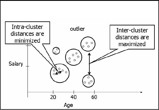
Clustering: Min-Max
Distance
Finding
groups of objects such that
the objects in a group are similar
(or related) to one
another
and dissimilar
from (or unrelated to)
the objects in other groups
e.g. using K-Means.
Figure-31.2:
Min-Max Distance
Now we talk
about "distance" which here
means that there must be
some measure of telling
how
much similar or
dissimilar a record is form another
e.g. height, GPA salary are
examples of a
258

single attribute. So
there should be a mechanism of
measuring the similarity or
dissimilarity. We
have
already discussed clustering
ambiguities, so when clusters are
formed in unsupervised
clustering,
the points having smaller
intracluster distances should fall in a
single cluster and
inter
clustering
distance between any two
clusters should be greater.
For example, consider the
age and
salary
attributes of employees as shown in
Figure 31.2. Every point here
corresponds to a single
employee
i.e. a single record. Look
at the cluster around age
60, these might be retired
people
getting pensions
only. There is another
cluster at the age of 68,
these are the people
aged enough
but still
may stick to their
organizations. The thing to
understand here is that as
the age increases
the
salary increases but when
people get retirements their
salaries fall. The first
clus ter in the
diagram shows
young people with low
salaries. There is another
cluster too that shows old
people
with
low salaries. There is also
a cluster showing young and high
salary, called outliers. These
are
the
people who might be working in their
"Abba Jee's "company. So u
must have understood
outliers,
inter-cluster and intra-cluster
distances.
How
Clustering works?
§
Works on
some notion of natural association in
records (data) i.e. some
records are more
similar to
each other than the
others.
§
This
concept of association must be
translated into some sort of
numeric measure of
the
degree of
similarity.
§
It works by
creating a similarity matrix by
calculating pair-wise distance measure
for n
x
m data
matrix.
§
Similarity matrix if
represented as a graph can be
clustered by:
§ Partitioning
the graph
§ Finding
cliques in the graph
In clustering
there has to be the notion
of association between records
i.e. which records
are
associated
with other records in the
data set. You have to
find that association. There
has to be a
distance
matrix and you have to map
that on the association. You
may be able to quantify
the
association
among closely related
records. Remember that all
the attributes may not be
numeric,
attributes
may be non numeric as well e.g.
someone's appointment, job title,
likes and dislikes
are
all non numeric
attributes. Thus taking these numeric and
non numeric attributes you have to
make an
association measure which
will associate records. When
such a measure is formed,
it
will reflect
the simila rity between
records. On the basis of
that similarity a similarity
matrix will
be built (one
way clustering) that will be
square, symmetric having
same diagonal value 1.
Since
we are
using Pearson's coefficient
the values in the matrix will be
between -1 and +1.
For
opposing items
when one is rising and
the other is falling, the
correlation will be -1. For
those
items
that fall and rise
simultaneously, there will be a
correlation of +1 and if no correlation
then
0. For
the sake of simplicity, it is represented
as a binary matrix i.e. if correlation greater
than 0.5
it will be
represented with 1. If correlation less
than 0.5, it will be
represented with 0. Thus in
this
way
the similarity matrix which
was real is transformed into the
binary matrix. Question ar
ises
where is the
clustering? Now assume that
your binary matrix represents a graph. As
you might
have
studied that a graph can be
represented as a matrix. So we utilize
some graph properties
for
performing
clustering. We can use two
techniques. One is the graph
partitioning in which
the
graph is portioned in
such a way that the
connectivity among vertices in the
partition is higher
than
across the partitions. Thus we
performed clustering through graph partitioning.
Another
technique
called clique detection can
also be used but we will
not go into the
details.
259
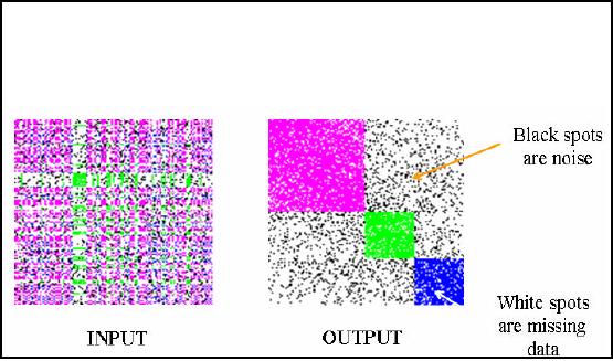
One-way
clustering
Clustering all
the rows or all the
columns simultaneously.
Gives a
global view.
Figure
32.3: One-way clustering
example
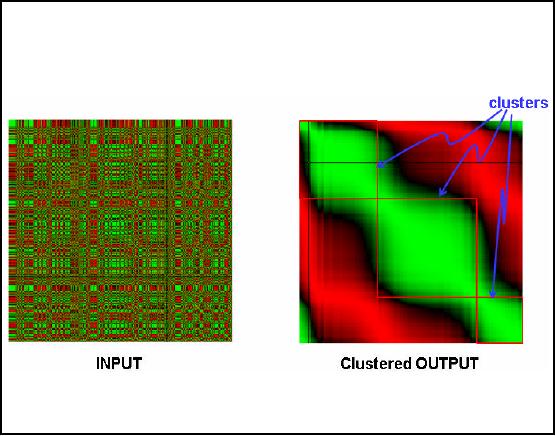
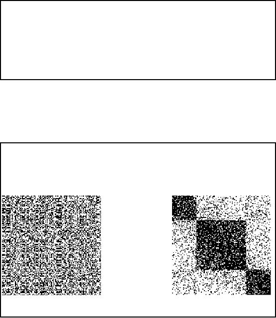
Now I
will give you a real example of
one way clustering. A data
matrix is taken and
intentionally
put 3 clusters in that. Then
similarity matrix is formed
from data matrix and
the
clusters
are also color coded
for better understanding.
The similarity matrix is then
randomly
permuted
and some also is also
inserted. The final shape of
the matrix is as shown in Figure
32.3
and
will be used as input to the
clustering technique. You
can see some black
and white points.
White points
represent missing values which
can either be in data or similarity
matrix. Black
points represent
noise i.e. those data values
which should not be present in the
data set. Now I
apply my own
indigenous technique for performing
clustering this input
similarity matrix. The
result is
shown as output in Figure 32.3. Here
you can see very
well defined clusters and
all these
clusters
are clearly visible and
distinguishable because of color coding.
Remember that in
previous
lecture it was stated that
good DM techniques should be robust. So
our technique
applied
here is highly robust
because it worked fairly well even in
the presence of noise.
Genetic
algorithms that
we discussed previously are not
robust because they do not
work well in the
presences of
noise.
260
Data Mining
Agriculture data
Created a
similarity matrix using farm area,
cotton variety and pesticide
used.
Color
coded the matrix, with green
assigned to +1 and red to
-1.
Large farmers
using fewer varieties of
cotton and fewer
pesticides.
Small
farmers using left
-overs.
Figure-32.4:
Data Mining Agriculture data
In the previous
slide the example was
based on simulated data where
the clusters were
intentionally
inserted into the data.
Now we will consider a real
world example where agricultural
data
has been use. The
data, pest scouting data,
has been taken from
department of pest
warning
Punjab
for the year 2000 and
2001. Some of the attributes
like farm area, cotton
variety cultivated
and
pesticide used are selected.
Using these and some other
attributes a similarity matrix has
been
formed
based on Pearson's Correlation.
The matrix thus has values
between +1 and -1 for
better
understanding
color coding is used and
most positive i.e. +1 is
represented with green and
-1 is
represented
with red color. Furthermore, as these
values proceed towards zero
from either side,
the
colors are darkened
accordingly.
Input
matrix in Figure 32.4 shows
the color coded similarity
matrix. We can say that
data
visualization
has been performed here
since we can see the
relationship among records which
are
around 600 to 700 in
number. Otherwise it is not possible to
visualize such a big table
in a single
sight.
Now when the clustering
technique is applied in this input
matrix the result is shown
in
Figure
32.4 as clustered output. Here we
see that the green
points have grouped together
i.e. those
points
having high correlation or records
having more association have
grouped together. This is
what we needed
and points with low
association i.e. red color
points have separated. Here
one
thing is
important that the input and
the output matrices are identical
except that the order of
rows
and
columns has been changed.
The cluster in the output
matrix is also present in the input
matrix
but is not
visible only because of reordering.
Interesting enough if you search the
world's greatest
261
and number
one search engine Google
for
key words "data mining" and
"agriculture", it results
in 4 lakh
hits
and 4th hit being the
work done by me.
So what is the
significance of doing all what mentioned
above? The results showed
that which
type of
farmers small or big use
what sort of varieties, which pesticide
and in what quantity etc.
The
information is useful from marketing
point of view and can be
used by pesticide
manufacturing
companies, seed breeders and
so on for m king effective
decisions about their
a
target
market.
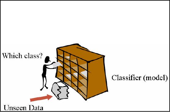
Classification
Examining the
features of a newly presented
object and assigning it to
one of a predefined set
of
classes.
Example:
Assigning keywords to
articles. Classification of credit applicants.
Spotting fraudulent insurance
claims.
Figure-32.5:
Classification
In one of
the previous slide took and
overview of classification. Now we will
discuss it in detail
but before
this have a look at the
analogy in Figure 32.5. Here you
can see a person is standing
by
a rack
that is boxed. It may also
be called as a pigeon hole
box. Each box in
the rack represents a
class
while the whole rack is a
classifier model. Alongside the
rack, there also lies a
documents
filled
bag which is the unseen
data. It means that it is unknown
that to which box or class
these
documents
belong. So using the
classification technique and
the built in model each
document is
assigned to
its respective box or class in
the rack. Thus for
performing classification, you
must
have a
classification model in place and
also the classes must be
known a priori. You must
know
the
number of classes and there
attributes as well i.e. by
looking at the data
properties of any
picked
document, the classification
process will know the
box/class of the document
that it
belongs
to. Thus in this way classification is
performed. The classification can be used
for
customer
segmentation, to detect fraudulent
transactions and issues
related to money laundering
and
the list goes on.
262
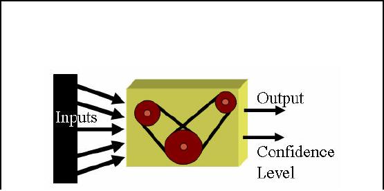
How
Classification work?
§
It works by
creating a model based on known
facts and historical data by
dividing into
training
and test set.
§
The model is
built using the test
set where the class is known
and then applying it to
another
situation where the class is
unknown.
Figure-32.6:
How Classification works?
With
understanding of classification by
analogy in previous slide,
lets discuss formally how
the
classification
process actually works. First of
the available data set is
divided int o two parts,
one
is called test
set and the other is called
the training set. We pick
the training set and a model
is
constructed
based on known facts,
historical data and class
properties as we already know
the
number of
classes. After building the
classification model, every record of
the test set is posed
to
the
classification model which decides
the class of the input
record. Thus class label is given
as
the output of
the model as shown in Figure 32.6. It
should be noted that you
know the class
for
each record in
test set and this fact is
used to measure the accuracy
or confidence level of the
classification
model. You can find
accuracy by
Accuracy or
confidence level = matches/ total
number of matches
In simple words,
accuracy is obtained by divid
ing number of correct assignments by
total number
of assignemnets
by the classification
model.
263
Classification
: Use in Prediction
gure-32.7:
Classification Process- Model
Construction
Here we will
discuss how classification
can be used for prediction.
Before going into the
details
we must
try to understand what if we predict?
Does data mining really beneficial? In
one of our
previous
lectures, we talked about
assigning priorities to data
sets in the context of data
qua lity.
We also
talked about group
priorities and group
precedence. The concept was
that if your data
comes
from two different sources
and in one of those sources
customers have told their
gender
and if
data passes through right
processes then you the
customer gender (high data
quality).
However,
there might be some
customers which might not
have specified or mentioned
their
gender. So
the quality of such a data
is questionable.
A possible
solution to the problem of missing
gender could be to assign gender on
the basis of
names.
However, there might be some
confusing names on the basis of
which gender can not
be
assigned
like Firdous, Riffat, and
Shaheen etc. In such a
situation we can use data
mining for data
cleansing.
So lets have a look at
how we form a classification model
using a customer data
set
and
then using that model for
the identification of the
unspecified gender which is
mostly correct.
So,
two aspects data cleansing
and classification are being covered here
simultaneously.
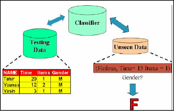
First of all w e
will look in to the details
of model construction process. Figure
32.8 shows a view
of the
training data set. Here you
can see 6 records and 4
attributes. Time means how
much time a
customer
spends during the shopping
process. Items column refers to how
many items a customer
buys
while gender shows either
the customer male or female.
This training set is the
input to
classification
algorithms which automatically analyze
the input data and
construct a model or
classifier.
The model could be a mathematical
expression or a rule such as if
then statement. The
model in our
case is a rule that if the
per item minutes for any
customer is greater or equal
than 6
than
the customer is female else a
male i.e.
264
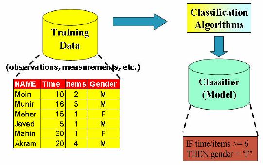
IF
Items/Time >=
6
Then
Gender=
`F'
else
Gender =
`M'
The
above rule is based on the
common notion that females
spend more time during shoping
than
male
customers. Exceptions can be
there and are treated as
outliers.
Figure-32.8:
Classification model
construction
Now
once the model is built we
have to test the accuracy of
our classification model. For
this
purpose we
take or test data set.
Three randomly picked test
data records have been shown
in
Figure
32.7. It is not the case
that our test data
contains only three records,
here we have taken
just
three records for the
sake of simplicity and let you
understand the concept. We
already know
the
classes of the test data
set records i.e. we know
their gender. The fact will
be utilized to
measure
the accuracy of our model. So we
will pick each of the three
records one after
another
and
put into the classifier.
Since for the first
record the ration is greater
than 6 meaning that
our
model will
assign it to the female class,
but that may be an exception
or noise. The second and
the
third
records are as per rule. Thus,
the accuracy of our model is
2/3 i.e. .66%. In other words
we
can
say the confidence level of
our classification model is 66%.
The accuracy may change as
we
add
more data. Now unseen
data is brought into the
picture. Suppose the re is a record
with name
Firdous, time
spent 15 minutes and 1 item
purchased. We predict the gender by
using our
classification
model and as per our model
the customer is assigned `F'
(15/1=15 which is greater
than 6). Thus we
can easily predict the
missing data with some
reasonable accuracy
using
classification.
265
Clustering
vs. Cluster Detection
In one
-way clustering, reordering of rows (or
columns) assembles
clusters.
If the
clusters are NOT assembled,
they are very difficult to
detect.
Once
clusters are assembled, they
can be detected automatically,
using classical techniques
such
as K
-means.
The
difference between clustering
and clustering is an important thing to
understand. Basically
these
are two different concepts,
mostly misperceived by novice data
miners. First you
cluster
your
data and then detect
clusters in the clustered
data. If you take unclustered
input and try to
find
clusters, you may get some
clusters or some part of a
cluster no use of that. Thus
until and
unless
clustering is performed, cluster
detection is useless. The
purpose here is to let
you
understand
and remember the two
mostly confusing concepts which
are poles apart.
Clustering
vs. Cluster Detection:
EXAMPLE
Can you
SEE the cluster in
Fig-A?
How
about Fig-B?
A
B
Figure-32.9:
Clustering vs. Cluster Detection
EXAMPLE
For
better understanding consider
the example in Figure 32.9.
Can you tell the number of
clusters,
if there, by
looking at Figure 32.9(A)? No you
can't tell except that
every point is a cluster
but
that is
useless information. Cluster
detection in Figure 32.9(A) is thus a
very difficult task
as
clusters
here are not visible.
When clusters are detected,
its not necessary that
the clusters are
visible as
computer has no eyes. The
clusters may be huge enough
that you can not even
display
or even if
displayed you can not visualize. So
cluster visualization is not that much a
problem.
Now
look at figure 32.9(B). The
three clusters here are
easily visible. We know that
the Figures A
and B
are identical except that reordering
has been performed on A in a scientific
manner using
266
our
own indigenous technique. Figure
32.9(B) is the clustered
output and when cluster
detection
will be
performed on B, three clusters
will successfully be detected. If A is
taken as input to the
cluster
detection algorithm instead of B, you
may end with nothing. There
is a misconception
among
new data miners that
cluster detection is a simple
task. They think that
using K-means is
everything.
This is not always the case,
k-means can not work always
. Can it work for
matrices
A and B? Wait
till last slide for
the answer.
The
K-Means
Clustering
§
Given
k, the
k-means
algorithm is
implemented in 4 steps:
§
Partition
objects into k nonempty
subsets
§
Compute seed
poin ts as the centroids of
the clusters of the current
partition. The
centroid is the
center (mean point) of the
cluster.
§
Assign
each object to the cluster
with the nearest seed
point.
§
Go back to
Step 2, stop when no more new
assignment.
Before
mentioning the strengths and
weaknesses of the k-means,
lets first discuss it
working. It is
implemented in
four steps.
Step 1:
In
the first step you assign
k
clusters in
your data set. Thus it's a
supervised technique as
you
must know the
number of classes
and
their
properties a
priori.
Step 2:
The
second step is to compute
the seed points or centroids
of your defined clusters
i.e.
which
value is a most representative
value of all the points in a
cluster. For the sake of
your
convenience, we
are talking about 2- D space, otherwise
k-means can work for
multidimensional
data
sets as well. The centroid
can be the mean of these
points, hence called
k-means.
Step 3:
In
this step you take the
distance of each point from
the cluster centroids or
means. On
the basis of a
predefined threshold value, it is decide
that which point belongs to
which cluster.
Step 4:
You
may repeat the above
steps i.e. you find the
means of newly formed
clusters then
find
the distances of all points
from those means and
clusters are reconfigured. The
process is
normally
repeated until some changes
occur in clusters and mostly
you get better
results.
267
The
K-Means
Clustering:
Example
A
B
1
1
0
0
9
9
8
8
7
7
6
6
5
5
4
4
3
3
2
2
1
1
0
0
1
0
1
2
3
4
5
6
7
8
9
1
0
1
2
3
4
5
6
7
8
9
0
0
1
1
9
9
8
8
7
7
6
6
5
5
4
4
3
3
2
2
1
1
0
0
0
1
2
3
4
5
6
7
8
9
1
0
1
2
3
4
5
6
7
8
9
1
0
0
D
C
Figure-32.10:
The K-Means
Clustering
Example
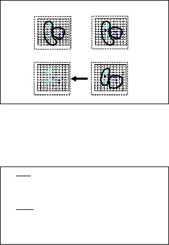
Consider
the example in the figure
32.10 for better
understanding k-means working. Figure
A
shows
two sets of color points
and the two colors
represent two different
classes. The polygons
drawn around
points in different clusters
signify the cluster
boundaries. Now at Figure B a
red
point
has come in each of the
two clusters. This is the
centroid or mean of the value in
that
cluster.
The next step is to measure
the distances of all the
points from each of these
centoirds. So
those
distances which are above
some threshold will go in a
cluster for each mean
point or
centroid.
Now look at the figure C,
here on the basis of
distances measured in the previous
step
new cluster
boundaries have been made. In
figure D the boundaries have
been removed and we
see
that a point has been
removed from one of the
clusters and added to the
other. As we will
repeat
the process, the result
will get more and
finer.
The
K-Means
Clustering:
Comment
§
Strength
§ Relatively
efficient: O (tkn), where
n
is #
objects, k is # clusters,
and t is #
iterations.
Normally, k, t << n.
§
Often
terminates at a local
optimum. The
global
optimum may be
found using
techniques
such as: deterministic
annealing and
genetic
algorithms
§
Weakness
§ Applicable
only when mean
is defined,
then what about categorical
data?
§
Need to specify
k,
the
number
of
clusters, in advance
§
Unable to handle
noisy data and outliers
§
Not
suitable to discover clusters with
non-convex
shapes
268
At the
end of the lecture there
are some comments about
k-means:
1. K-means is a
fairly fast technique and
normally when terminates , then
clusters formed
are
fairly good.
2. It can
only work for data
sets where there is the
concept of mean (the answer to
the
question
posed in a few slides back).
If data is non numeric such as likes
dislikes, gender,
eyes
color etc. then how to
calculate means. So this is
the first problem with
the
technique.
3. Another
problem or limitation of the
technique is that you have to specify
the number of
cluster in
advance.
4. The
third limitation is that it is not a
robust technique as it not works
well in presence of
noise.
5. The
last problem is that the
clusters found by k-means have to be
convex i.e. if you draw
a polygon
and join parameters of any
two points in that polygon,
that line goes out of
the
cluster
boundaries.
269
Table of Contents:
- Need of Data Warehousing
- Why a DWH, Warehousing
- The Basic Concept of Data Warehousing
- Classical SDLC and DWH SDLC, CLDS, Online Transaction Processing
- Types of Data Warehouses: Financial, Telecommunication, Insurance, Human Resource
- Normalization: Anomalies, 1NF, 2NF, INSERT, UPDATE, DELETE
- De-Normalization: Balance between Normalization and De-Normalization
- DeNormalization Techniques: Splitting Tables, Horizontal splitting, Vertical Splitting, Pre-Joining Tables, Adding Redundant Columns, Derived Attributes
- Issues of De-Normalization: Storage, Performance, Maintenance, Ease-of-use
- Online Analytical Processing OLAP: DWH and OLAP, OLTP
- OLAP Implementations: MOLAP, ROLAP, HOLAP, DOLAP
- ROLAP: Relational Database, ROLAP cube, Issues
- Dimensional Modeling DM: ER modeling, The Paradox, ER vs. DM,
- Process of Dimensional Modeling: Four Step: Choose Business Process, Grain, Facts, Dimensions
- Issues of Dimensional Modeling: Additive vs Non-Additive facts, Classification of Aggregation Functions
- Extract Transform Load ETL: ETL Cycle, Processing, Data Extraction, Data Transformation
- Issues of ETL: Diversity in source systems and platforms
- Issues of ETL: legacy data, Web scrapping, data quality, ETL vs ELT
- ETL Detail: Data Cleansing: data scrubbing, Dirty Data, Lexical Errors, Irregularities, Integrity Constraint Violation, Duplication
- Data Duplication Elimination and BSN Method: Record linkage, Merge, purge, Entity reconciliation, List washing and data cleansing
- Introduction to Data Quality Management: Intrinsic, Realistic, Orrs Laws of Data Quality, TQM
- DQM: Quantifying Data Quality: Free-of-error, Completeness, Consistency, Ratios
- Total DQM: TDQM in a DWH, Data Quality Management Process
- Need for Speed: Parallelism: Scalability, Terminology, Parallelization OLTP Vs DSS
- Need for Speed: Hardware Techniques: Data Parallelism Concept
- Conventional Indexing Techniques: Concept, Goals, Dense Index, Sparse Index
- Special Indexing Techniques: Inverted, Bit map, Cluster, Join indexes
- Join Techniques: Nested loop, Sort Merge, Hash based join
- Data mining (DM): Knowledge Discovery in Databases KDD
- Data Mining: CLASSIFICATION, ESTIMATION, PREDICTION, CLUSTERING,
- Data Structures, types of Data Mining, Min-Max Distance, One-way, K-Means Clustering
- DWH Lifecycle: Data-Driven, Goal-Driven, User-Driven Methodologies
- DWH Implementation: Goal Driven Approach
- DWH Implementation: Goal Driven Approach
- DWH Life Cycle: Pitfalls, Mistakes, Tips
- Course Project
- Contents of Project Reports
- Case Study: Agri-Data Warehouse
- Web Warehousing: Drawbacks of traditional web sear ches, web search, Web traffic record: Log files
- Web Warehousing: Issues, Time-contiguous Log Entries, Transient Cookies, SSL, session ID Ping-pong, Persistent Cookies
- Data Transfer Service (DTS)
- Lab Data Set: Multi -Campus University
- Extracting Data Using Wizard
- Data Profiling