MARGINAL UTILITY AND CONSUMER CHOICE:COST-OF-LIVING INDEXES

<< Note it is repeated:Consumer Preferences, Revealed Preferences

Review of Consumer Equilibrium:INDIVIDUAL DEMAND, An Inferior Good >>

Microeconomics ECO402

Lesson 9

MARGINAL UTILITY AND CONSUMER CHOICE

Marginal utility

measures the additional satisfaction obtained from consuming one additional unit of a

good.

Marginal Utility: An Example

The marginal utility derived from increasing from 0 to 1 units of food might be 9

Increasing from 1 to 2 might be 7

Increasing from 2 to 3 might be 5

Observation: Marginal utility is diminishing

Diminishing Marginal Utility

The principle of diminishing marginal utility states that as more and more of a good is

consumed, consuming additional amounts will yield smaller and smaller additions to

utility.

Relationship of Total and Marginal Utility

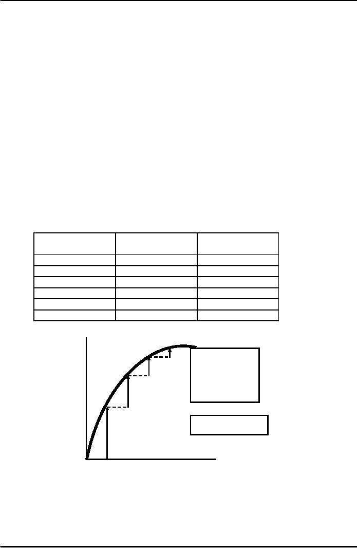
Diminishing Marginal Utility: An Example

Quantity of good

Total utility

Marginal utility

consumed

Utility

Total utility of

consuming a certain

amount is equal to

the sum of the

marginal utilities up

to the point

Total utility increases

at a decreasing rate

Quantity

Microeconomics ECO402

Marginal Utility

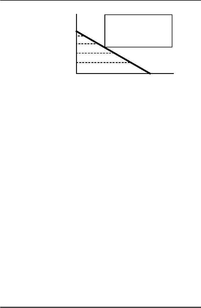
The fact that total utility

increases at a decreasing

rate is shown by negative

slope of marginal utility

curve

Quantity

Marginal Utility and

Consumer Choice

Marginal Utility and the Indifference Curve

If consumption moves along an indifference curve, the additional utility derived from an

increase in the consumption of one good, food (F), must balance the loss of utility from

the decrease in the consumption in the other good, clothing (C).

Formally:

0 = MUF (ΔF) + MUC (ΔC)

Rearranging:

- (ΔC/ ΔF) = MUF / MUC

Because:

- ( ΔC / ΔF ) = MRS of F for C

MRS = MUF/MUC

When consumers maximize satisfaction the:

MRS = PF/PC

Since the MRS is also equal to the ratio of the marginal utilities of consuming F and C, it

follows that:

MUF/MUC = PF/PC

Which gives the equation for utility maximization?

MU F / PF = MU C / PC

Total utility is maximized when the budget is allocated so that the marginal utility per dollar

of expenditure is the same for each good.

This is referred to as the equal marginal principle.

Microeconomics ECO402

Gasoline Rationing

In 1974 and again in 1979, the government imposed price controls on gasoline.

This resulted in shortages and gasoline was rationed.

Non-price rationing is an alternative to market rationing.

Under one form everyone has an equal chance to purchase a rationed good.

Gasoline is rationed by long lines at the gas pumps.

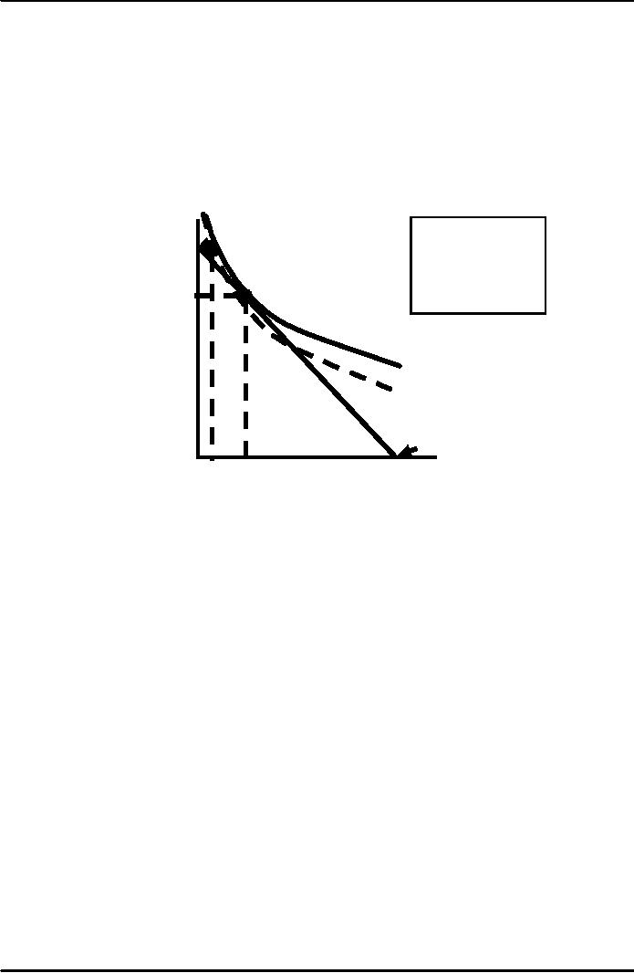
Rationing hurts some by limiting the amount of gasoline they can buy.

This can be seen in the following model.

It applies to a woman with an annual income of $20,000.

Spending

on other

With a limit of

goods ($) 20,000

2,000 gallons,

the consumer moves

18,00

to a lower

indifference curve

15,00

(lower level of utility).

Gasoline

2,00 5,00

20,00

(gallons per year)

COST-OF-LIVING INDEXES

The CPI is calculated each year as the ratio of the cost of a typical bundle of consumer

goods and services today in comparison to the cost during a base period.

Example

Two sisters, Raheela and Sarah, have identical preferences.

Sarah began college in 1987 with a $500 discretionary budget.

In 1997, Raheela started college and her parents promised her a budget that was

equivalent in purchasing power.

Price of books

$20/book

$100/book

Number of books

Price of food

$2.00/lb

$2.20/lb

Pounds of food

100

300

Expenditure

$500

$1,260

· Sarah' Expenditure

$500=100 lbs of food x $2.00/lb +15 books x $20/book

Raheela' Expenditure for Equal Utility

$1,260=300 lbs of food x $2.20/lb +6 books x $100/book

Microeconomics ECO402

The ideal cost-of-living adjustment for Raheela is $760.

The ideal cost-of-living index is $1,260/$500 = 2.52 or 252.

This implies a 152% increase in the cost of living.

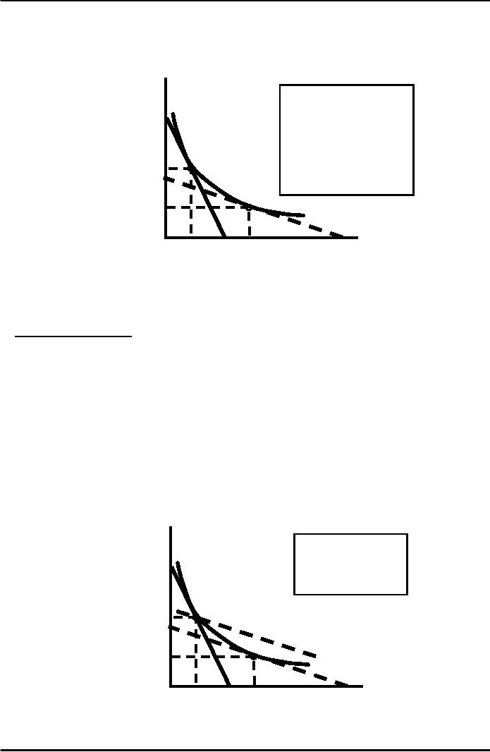
Books

(per

For Raheela to achieve

quarter)

the same level of utility

as Sarah, with the higher

prices, her budget must

be sufficient to allow her

to consume the bundle

shown by point B.

Food

(lb./quarter)

0 50 100 200 250 300 350 400 450 500 550 600

The ideal cost of living index represents the cost of attaining a given level of utility at current

(1997) prices relative to the cost of attaining the same utility at base (1987) prices.

To do this on an economy-wide basis would entail large amounts of information.

Price indexes, like the CPI, use a fixed consumption bundle in the base period. Called a

Laspeyres price index.

The Laspeyres index tells us:

The amount of money at current year prices that an individual requires to purchase the

bundle of goods and services that was chosen in the base year divided by the cost of

purchasing the same bundle at base year prices.

Calculating Raheela's Laspeyres cost of living index

Setting the quantities of goods in 1997 equal to what were bought by her sister, but

setting their prices at their 1997 levels result in an expenditure of

$1,720 (100 x 2.20 + 15 x $100)

Her cost of living adjustment would now be $1,220.

The Laspeyres index is:

$1,720/$500 = 344.

This overstates the true cost-of-living increase.

Books

(per quarter)

Using the Laspeyres

index results in the

budget line shifting

up from I2 to I3.

Food

(lb./quarter)

0 50 100 200 250 300 350 400 450 500 550 600

Microeconomics ECO402

What Do You Think?

Does the Laspeyres index always overstate the true cost-of-living index?

Yes!

The Laspeyres index assumes that consumers do not alter their consumption patterns

as prices change.

By increasing purchases of those items that have become relatively cheaper, and

decreasing purchases of the relatively more expensive items consumers can achieve

the same level of utility without having to consume the same bundle of goods.

The Paasche Index

Calculates the amount of money at current-year prices that an individual requires to

purchase a current bundle of goods and services divided by the cost of purchasing the

same bundle in the base year.

Comparing the Two Indexes

Suppose:

Two goods: Food (F) and Clothing (C)

Comparing the Two Indexes

Let:

· P & P be current year prices

· P & P be base year prices

· F & C be current year quantities

· F & C be base year quantities

Both indexes involve ratios that involve today's current year prices, PFt and PCt.

However, the Laspeyres index relies on base year consumption, Fb and Cb.

Whereas, the Paasche index relies on today's current consumption, Ft and Ct .

Then a comparison of the Laspeyres and Paasche indexes gives the following equations:

LI = --P-Ft-F-b----P-Ct-Cb----

- - - + - - ---

PFb Fb + PCb Cb

PI = --P---F--+---C----------

- Ft - t - P -t Ct

PFb Ft + PCb Ct

Sarah

(1990)

· Cost of base-year bundle at current prices equals

$1,720 (100 lbs x $2.20/lb + 15 books x $100/book)

· Cost of same bundle at base year prices is

$500 (100 lbs x $2.00/lb + 15 books x $20/book)

Sarah (1990)

$1, 720

LI =

= 344

$500

· Cost of buying current year bundle at current year prices is

$1,260 (300 lbs x $2.20/lb + 6 books x $100/book)

Microeconomics ECO402

· Cost of the same bundle at base year prices is

$720 (300 lbs x $2/lb + 6 books x $20/book)

$1,260

PI =

= 175

$720

The Paasche index will understate the cost of living because it assumes that the individual

will buy the current year bundle in the base year.

Table of Contents: