CONSUMER PREFERENCES:Budget Constraints, Consumer Choice

<< Consumer Behavior:Consumer Preferences, Indifference curves

Note it is repeated:Consumer Preferences, Revealed Preferences >>

Microeconomics ECO402

LESSON 7

CONSUMER PREFERENCES

Utility

Numerical score representing the satisfaction that a consumer gets from a

given market basket.

If buying 3 copies of Microeconomics makes you happier than buying one shirt,

then we say that the books give you more utility than the shirt.

Utility Functions

Assume: The utility function for food (F) and clothing (C)

U(F,C) = F + 2C

Market Baskets:

F units

C units

U (F, C) = F + 2C

8 + 2(3) = 14

6 + 2(4) = 14

4 + 2(4) = 12

The consumer is indifferent to A & B

The consumer prefers A & B to C

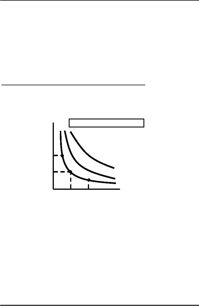
Utility Functions & Indifference Curves

Clothing

(units

per week)

Assume: U = FC

Market Basket

U = FC

25 = 2.5(10)

25 = 5(5)

25 = 10(2.5)

U3 = 100 (Preferred to

U2 = 50 (Preferred to

U1 = 25

Food

(units per week)

Ordinal Versus Cardinal Utility

Ordinal Utility Function: places market baskets in the order of most preferred

to least preferred, but it does not indicate how much one market basket is

preferred to another.

Cardinal Utility Function: utility function describing the extent to which one

market basket is preferred to another.

Ordinal Versus Cardinal Rankings

The actual unit of measurement for utility is not important.

Therefore, an ordinal ranking is sufficient to explain how most individual

decisions are made.

Budget Constraints

Preferences do not explain all of consumer behavior.

Budget constraints also limit an individual's ability to consume in light of the prices they

must pay for various goods and services.

The Budget Line

The budget line indicates all combinations of two commodities for which total

money spent equals total income.

Microeconomics ECO402

The Budget Line

Let F equal the amount of food purchased, and C is the amount of clothing.

Price of food = Pf and price of

clothing = Pc

Then Pf F is the amount of money spent on food, and Pc C is the amount of

money spent on clothing.

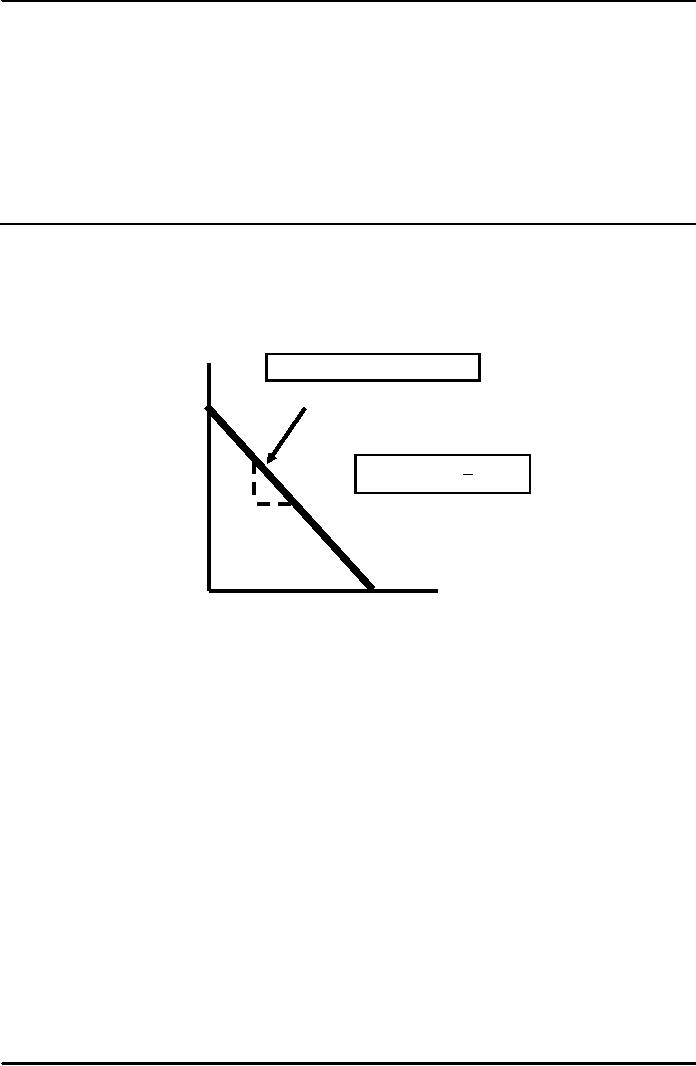
The budget line then can be written:

PFF + PCC = I

Market Basket

Food (F)

Clothing (C)

Total Spending

Pf = ($1)

Pc = ($2)

PfF + PcC = I

$80

Clothing

Pc = $2

Pf = $1

I = $80

(units

per week)

Budget Line F + 2C = $80

(I/PC) = 40

Slope = ΔC/ΔF = -

= - PF/PC

Food

80 = (I/PF) (units per week)

The Budget Line

As consumption moves along a budget line from the intercept, the consumer

spends less on one item and more on the other.

The slope of the line measures the relative cost of food and clothing.

The slope is the negative of the ratio of the prices of the two goods.

The slope indicates the rate at which the two goods can be substituted without

changing the amount of money spent.

The vertical intercept (I/PC), illustrates the maximum amount of C that can be

purchased with income I.

The horizontal intercept (I/PF), illustrates the maximum amount of F that can be

purchased with income I.

The Effects of Changes in Income and Prices

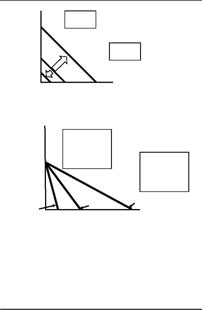
Income Changes

An increase in income causes the budget line to shift outward, parallel

to the original line (holding prices constant).

A decrease in income causes the budget line to shift inward, parallel to

the original line (holding prices constant).

Microeconomics ECO402

Clothing

A increase in

(units

income shifts

per week)

the budget line

outward

A decrease in

income shifts

the budget line

inward

(I =

$40

Food

120

160

(units per week)

Price Changes

· If the price of one good increases, the budget line shifts inward, pivoting

from the other good's intercept.

· If the price of one good decreases, the budget line shifts outward,

pivoting from the other good's intercept.

Clothing

An increase in the

(units

price of food to

per week)

$2.00 changes

the slope of the

budget line and

A decrease in the

rotates it inward.

price of food to

$.50 changes

the slope of the

budget line and

rotates it outward.

(PF = 1)

(PF = 1/2)

(PF = 2)

Food

120

160

(units per week)

The Effects of Changes in Income and Prices

Price Changes

· If the two goods increase in price, but the ratio of the two prices is

unchanged, the slope will not change.

· However, the budget line will shift inward to a point parallel to the

original budget line.

· If the two goods decrease in price, but the ratio of the two prices is

unchanged, the slope will not change.

· However, the budget line will shift outward to a point parallel to the

original budget line.

Consumer Choice

Consumers choose a combination of goods that will maximize the satisfaction they can

achieve, given the limited budget available to them.

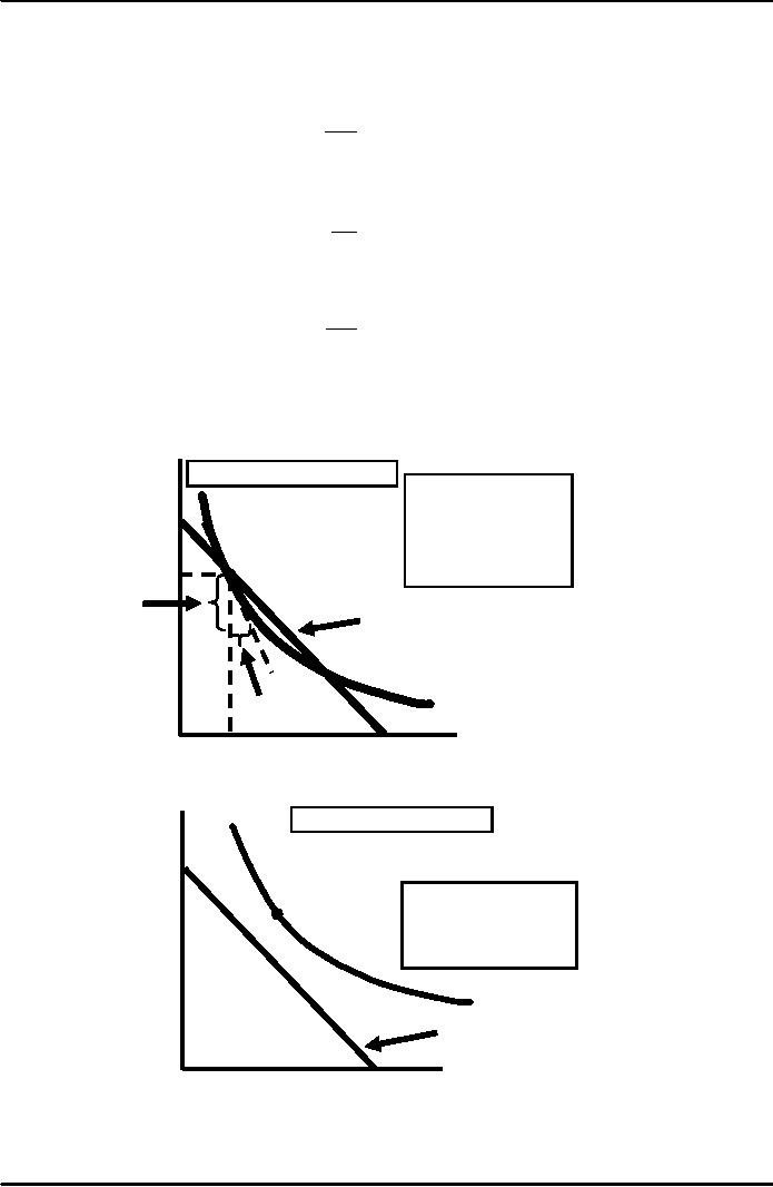
The maximizing market basket must satisfy two conditions:

1) It must be located on the budget line.

Microeconomics ECO402

2) Must give the consumer the most preferred combination of goods and

services.

Recall, the slope of an indifference curve is:

ΔC

MRS = -

ΔF

Further, the slope of the budget line is:

Slope = -

Therefore, it can be said that satisfaction is maximized where:

M RS =

It can be said that satisfaction is maximized when marginal rate of substitution (of F

and C) is equal to the ratio of the prices (of F and C).

Clothing

Pc = $2

Pf = $1

I = $80

(units per

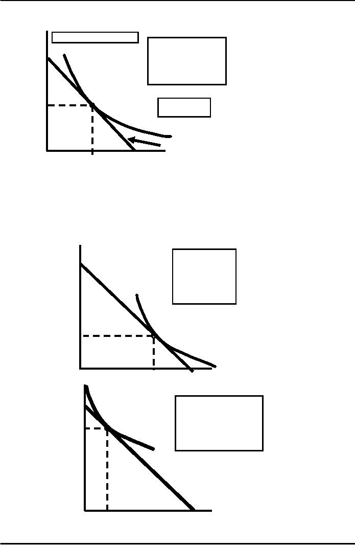
Point B does not

week)

maximize satisfaction

because the

MRS (-(-10/10) = 1

is greater than the

price ratio (1/2).

-10C

Budget

+10

Food (units per week)

Clothing

(units per

Pc = $2

Pf = $1

I = $80

week)

Market basket D

cannot be attained

given the current

budget constraint.

Budget

Food (units per week)

Microeconomics ECO402

Clothing

(units per

Pc = $2

Pf = $1

I = $80

week)

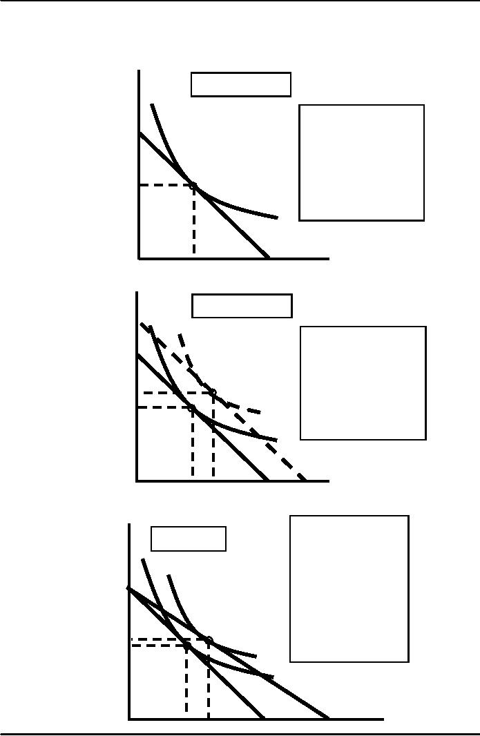
At market basket A

the budget line and the

indifference curve are

tangent and no higher

level of satisfaction

can be attained.

At A:

MRS =Pf/Pc = .5

Budget

Food (units per week)

Designing New Automobiles (II)

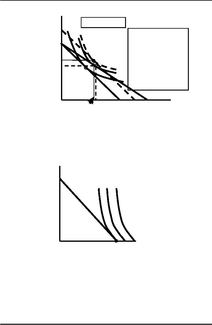
Consider two groups of consumers, each wishing to spend $10,000 on the

styling and performance of cars.

Each group has different preferences.

By finding the point of tangency between a group's indifference curve and the

budget constraint auto companies can design a production and marketing plan.

Styling

These consumers

$10,000

are willing to trade

off a considerable

amount of styling

for some additional

performance

$3,000

$7,000

$10,000 Performance

Styling

These consumers

$10,000

are willing to trade

off a considerable

amount of

$7,000

performance for

some additional

styling

$10,000 Performance

$3,000

Microeconomics ECO402

Decision making & Public Policy

Choosing between a non-matching and matching grant to fund police

expenditures

Private

Non-matching Grant

Expenditures ($)

Before Grant

· Budget line: PQ

·A: Preference maximizing

market basket

·Expenditure

·OR: Private

·OS: Police

Police

Expenditures ($)

Private

Expenditures ($)

Non-matching Grant

After Grant

· Budget line: TV

·B: Preference maximizing

market basket

·Expenditure

·OU: Private

·OZ: Police

Police

Expenditures ($)

Private

Before Grant

Expenditures ($)

· Budget line: PQ

Matching Grant

· A: Preference maximizing

market basket

After Grant

·C: Preference maximizing

market basket

Expenditures

·OW: Private

·OX: Police

Police ($)

Microeconomics ECO402

Private

Expenditures ($)

Matching Grant

Non-matching Grant

·Point B

·OU: Private expenditure

·OZ: Police expenditure

Matching Grant

·Point C

·OW: Private expenditure

U1 ·OX: Police expenditure

Police ($)

Corner Solution

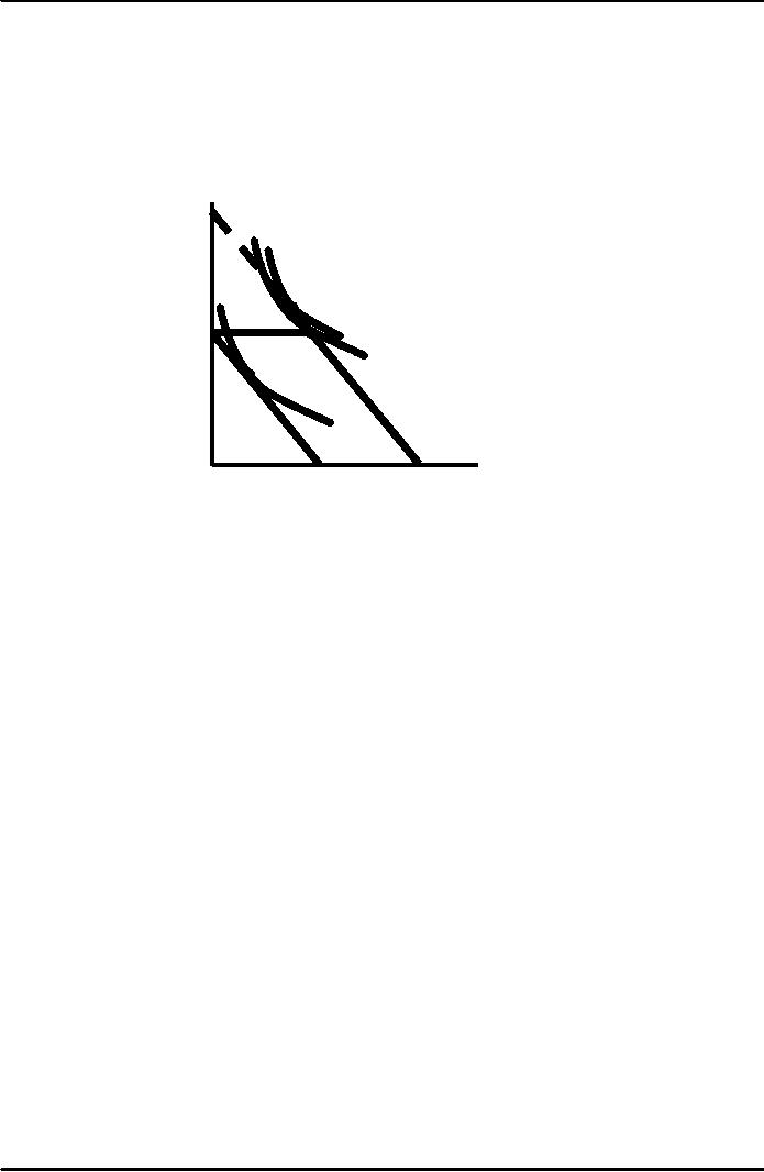
A corner solution exists if a consumer buys in extremes, and buys all of one

category of good and none of another.

· This exists where the indifference curves are tangent to the horizontal

and vertical axis.

MRS is not equal to PA/PB

Frozen

Yogurt

(cups

monthly) A

A corner solution

exists at point B.

Ice Cream (cup/month)

A Corner Solution

At point B, the MRS of ice cream for frozen yogurt is greater than the slope of the

budget line.

This suggests that if the consumer could give up more frozen yogurt for ice cream

he would do so.

However, there is no more frozen yogurt to give up!

When a corner solution arises, the consumer's MRS does not necessarily equal the

price ratio.

In this instance it can be said that:

MRS ≥ PIceCream / PFrozen Yogurt

Microeconomics ECO402

If the MRS is, in fact, significantly greater than the price ratio, then a small

decrease in the price of frozen yogurt will not alter the consumer's market

basket.

A college Trust Fund

Suppose Jane Doe's parents set up a trust fund for her college education.

Originally, the money must be used for education.

If part of the money could be used for the purchase of other goods, her

consumption preferences change.

A College Trust Fund

Other

Consumption

($)

A: Consumption before the trust fund

The trust fund shifts the budget line

B: Requirement that the trust fund

must be spent on education

C: If the trust could be spent on

other goods

Education ($)

Table of Contents: