 |
The Technology of Production:Production Function for Food |
| << PREFERENCES TOWARD RISK:Reducing Risk, The Demand for Risky Assets |
| Production with Two Variable Inputs:Returns to Scale >> |

Microeconomics
ECO402
VU
Lesson
16
Introduction
Our
focus is the supply
side.
The
theory of the firm will
address:
How a firm
makes cost-minimizing production
decisions
How cost
varies with output
Characteristics of
market supply
The
Technology of Production
The
Production Process
Combining
inputs or factors of production to
achieve an output
Categories
of Inputs (factors of
production)
Labor
Materials
Capital
Production
Function:
Indicates the
highest output that a firm
can produce for every
specified combination of
inputs
given the state of
technology.
Shows what is
technically feasible when
the firm operates
efficiently.
The
production functions for two
inputs:
Q
= F(K,L)
Q
= Output, K = Capital, L =
Labor
For
a given technology
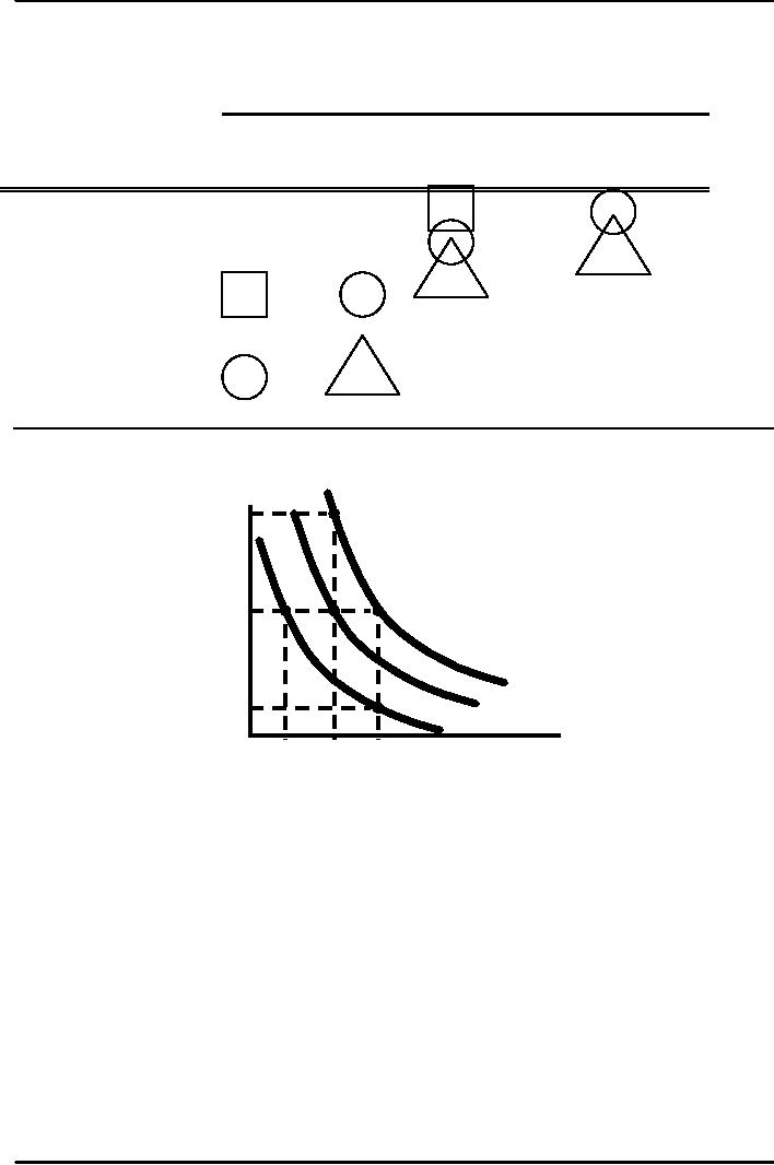
Isoquants
Assumptions
Food producer
has two inputs
�
Labor (L)
& Capital (K)
Observations:
1)
For any level of K, output
increases with more
L.
2)
For any level of L, output
increases with more
K.
3)
Various combinations of inputs
produce the same
output.
Isoquants
Curves showing
all possible combinations of
inputs that yield the
same output
78

Microeconomics
ECO402
VU
Production
Function for Food
Labor
Input
Capitan
Input
1
2
3
4
5
1
20
40
55
65
75
2
40
60
75
85
90
3
55
75
90
100
105
4
65
85
100
110
115
5
75
90
105
115
120
Production
with Two Variable Inputs
(L,K)
Capital
The
Isoquant Map
per
year
E
5
4
The
isoquants are derived
from
the production
function
for output of
3
A
B
C
of
55, 75, and
90.
2
Q3 =
90
D
Q2 =
75
1
Q1 =
55
1
2
3
4
5
Labor
per year
Input
Flexibility
The isoquants
emphasize how different input
combinations can be used
to
produce
the same output.
This
information allows the
producer to respond efficiently to
changes in the
markets
for inputs.
The
Short Run vs. long
Run
Short-run:
�
Period of
time in which quantities of
one or more production
factors cannot be
changed.
�
These
inputs are called fixed
inputs.
Long-run
�
Amount of
time needed to make all
production inputs
variable.
79

Microeconomics
ECO402
VU
Production
with One Variable Input
(Labor)
Amount
Amount
Total
Average
Marginal
of
Labor (L)
of
Capital (K)
Output
(Q)
Product
Product
0
10
0
---
---
1
10
10
10
10
2
10
30
15
20
3
10
60
20
30
4
10
80
20
20
5
10
95
19
15
6
10
108
18
13
7
10
112
16
4
8
10
112
14
0
9
10
108
12
-4
10
10
100
10
-8
Observations:
1)
With
additional workers, output
(Q) increases, reaches a
maximum, and
then
decreases.
2)
The average product of labor
(AP), or output per worker,
increases and
then
decreases.
Output
Q
AP
=
=
Labor
Input
L
3)
The
marginal product of labor
(MP), or output of the
additional worker,
increases
rapidly initially and then
decreases and becomes
negative..
80

Microeconomics
ECO402
VU
Δ
Output
ΔQ
MP
L =
=
Δ
Labor
Input
ΔL
Output
per
Month
D
112
Total
Product
C
60
A:
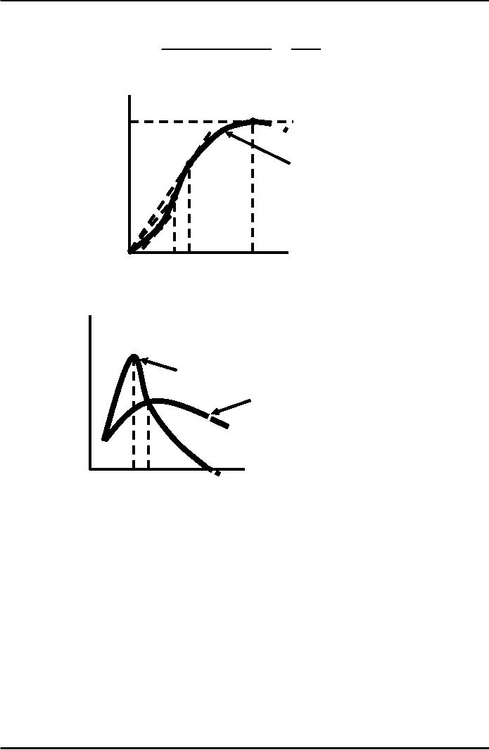
slope of tangent = MP
(20)
B
B:
slope of OB = AP (20)
C:
slope of OC= MP & AP
A
10
Labor per
Month
0
1
2
3
4
5
6
7
8
9
Output
Observations:
Left
of E: MP > AP & AP is
per
increasing
Month
Right
of E: MP < AP & AP is
decreasing
E:
MP = AP & AP is at its maximum
30
Marginal
E
Average
Product
20
10
0
1 2 3 4 5 6 7 8 9 10 Labor
per Month
Observations:
When MP = 0, TP is at
its maximum
When MP > AP, AP is
increasing
When MP < AP, AP is
decreasing
When MP = AP, AP is at
its maximum
81

Microeconomics
ECO402
VU
AP
= slope
of line from origin to a
point on TP,
lines b,
& c.
MP
= slope
of a tangent to any point on
the TP
line,
lines a & c.
The
Law of Diminishing Marginal
Returns
Output
Output
per
per
Month
Month
D
112
30
C
E
20
60
B
10
A
Labor
Labor
0
1 2 3 4 5 6 7 8 9 10 per
Month
0
1 2 3 4 5 6 7 8 9 10 per
Month
As the use of
an input increases in equal
increments, a point will be
reached at which
the
resulting additions to output
decreases (i.e. MP
declines).
When the
labor input is small, MP
increases due to
specialization.
When the
labor input is large, MP
decreases due to
inefficiencies.
The
Law of Diminishing Marginal
Returns
Can be used
for long-run decisions to
evaluate the trade-offs of
different plant
configurations
Assumes the
quality of the variable
input is constant
Explains a
declining MP,
not necessarily a negative
one
Assumes a
constant technology
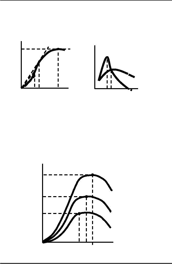
The
Effect of Technological
Improvement
Output
Labor
productivity
per
C
can
increase if there
time
are
improvements in
period
technology,
even though
100
any
given production
B
O3
process
exhibits
diminishing
returns to
labor.
A
O2
50
O1
Labor
per
time
period
0
1
2
3
4
5
6
7
8
9
10
82

Microeconomics
ECO402
VU
Malthus
and the Food
Crisis
Malthus
predicted mass hunger and
starvation as diminishing returns
limited agricultural
output
and the population continued
to grow.
Why
did Malthus' prediction
fail?
Index
of World Food Consumption
Per Capita
Year
Index
1948-1952
100
1960
115
1970
123
1980
128
1990
137
1995
135
1998
140
The
data show that production
increases have exceeded
population growth.
Malthus
did not take into
consideration the potential
impact of technology which
has allowed
the
supply of food to grow
faster than demand.
Technology
has created surpluses and
driven the price
down.
Question
If food
surpluses exist, why is
there hunger?
Answer
The cost of
distributing food from
productive regions to unproductive
regions and the
low
income
levels of the non-productive
regions.
Labor
Productivity
Total
Output
Average
Productivity =
Total
Labor Input
Labor
Productivity and the
Standard of Living
Consumption can
increase only if productivity
increases.
Determinants of
Productivity
�
Stock of
capital
�
Technological
change
83

Microeconomics
ECO402
VU
Labor
Productivity in Developed
Countries
United
United
France
Germany
Japan
Kingdom
States
Output
per Employed Person
(1997)
$54,507
$55,644
$46,048
$42,630
$60,915
Annual
Rate of Growth of Labor
Productivity (%)
1960-1973
4.75
4.04
8.30
2.89
2.36
1974-1986
2.10
1.85
2.50
1.69
0.71
1987-1997
1.48
2.00
1.94
1.02
1.09
Trends
in Productivity
1)
U.S. productivity is growing at a
slower rate than other
countries.
2)
Productivity growth in developed
countries has been
decreasing.
Explanations
for Productivity Growth
Slowdown
1)
Growth in the stock of
capital is the primary
determinant of the growth
in
productivity.
2)
Rate of capital accumulation in
the U.S. was slower
than other
developed
countries because the
others
were rebuilding after
WWII.
3)
Depletion of natural
resources
4)
Environment regulations
84
Table of Contents:
- ECONOMICS:Themes of Microeconomics, Theories and Models
- Economics: Another Perspective, Factors of Production
- REAL VERSUS NOMINAL PRICES:SUPPLY AND DEMAND, The Demand Curve
- Changes in Market Equilibrium:Market for College Education
- Elasticities of supply and demand:The Demand for Gasoline
- Consumer Behavior:Consumer Preferences, Indifference curves
- CONSUMER PREFERENCES:Budget Constraints, Consumer Choice
- Note it is repeated:Consumer Preferences, Revealed Preferences
- MARGINAL UTILITY AND CONSUMER CHOICE:COST-OF-LIVING INDEXES
- Review of Consumer Equilibrium:INDIVIDUAL DEMAND, An Inferior Good
- Income & Substitution Effects:Determining the Market Demand Curve
- The Aggregate Demand For Wheat:NETWORK EXTERNALITIES
- Describing Risk:Unequal Probability Outcomes
- PREFERENCES TOWARD RISK:Risk Premium, Indifference Curve
- PREFERENCES TOWARD RISK:Reducing Risk, The Demand for Risky Assets
- The Technology of Production:Production Function for Food
- Production with Two Variable Inputs:Returns to Scale
- Measuring Cost: Which Costs Matter?:Cost in the Short Run
- A Firm’s Short-Run Costs ($):The Effect of Effluent Fees on Firms’ Input Choices
- Cost in the Long Run:Long-Run Cost with Economies & Diseconomies of Scale
- Production with Two Outputs--Economies of Scope:Cubic Cost Function
- Perfectly Competitive Markets:Choosing Output in Short Run
- A Competitive Firm Incurring Losses:Industry Supply in Short Run
- Elasticity of Market Supply:Producer Surplus for a Market
- Elasticity of Market Supply:Long-Run Competitive Equilibrium
- Elasticity of Market Supply:The Industry’s Long-Run Supply Curve
- Elasticity of Market Supply:Welfare loss if price is held below market-clearing level
- Price Supports:Supply Restrictions, Import Quotas and Tariffs
- The Sugar Quota:The Impact of a Tax or Subsidy, Subsidy
- Perfect Competition:Total, Marginal, and Average Revenue
- Perfect Competition:Effect of Excise Tax on Monopolist
- Monopoly:Elasticity of Demand and Price Markup, Sources of Monopoly Power
- The Social Costs of Monopoly Power:Price Regulation, Monopsony
- Monopsony Power:Pricing With Market Power, Capturing Consumer Surplus
- Monopsony Power:THE ECONOMICS OF COUPONS AND REBATES
- Airline Fares:Elasticities of Demand for Air Travel, The Two-Part Tariff
- Bundling:Consumption Decisions When Products are Bundled
- Bundling:Mixed Versus Pure Bundling, Effects of Advertising
- MONOPOLISTIC COMPETITION:Monopolistic Competition in the Market for Colas and Coffee
- OLIGOPOLY:Duopoly Example, Price Competition
- Competition Versus Collusion:The Prisoners’ Dilemma, Implications of the Prisoners
- COMPETITIVE FACTOR MARKETS:Marginal Revenue Product
- Competitive Factor Markets:The Demand for Jet Fuel
- Equilibrium in a Competitive Factor Market:Labor Market Equilibrium
- Factor Markets with Monopoly Power:Monopoly Power of Sellers of Labor