 |
Review of Consumer Equilibrium:INDIVIDUAL DEMAND, An Inferior Good |
| << MARGINAL UTILITY AND CONSUMER CHOICE:COST-OF-LIVING INDEXES |
| Income & Substitution Effects:Determining the Market Demand Curve >> |
Microeconomics
ECO402
VU
Lesson
10
Review of
Consumer Equilibrium
Consumer
Preferences
Budget
Constraint
Consumer
Choices
INDIVIDUAL
DEMAND
Price
Changes
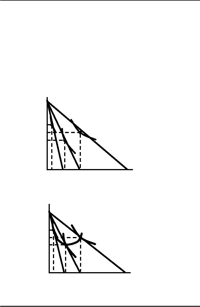
Using the
figures developed in the
previous chapter, the impact
of a change in the
price
of
food can be illustrated
using indifference
curves.
Effect
of a Price Change
Clothing
Assume:
(units
�I
= $20
per
1
month)
�P
= $2
C
A
6
U1
Three
separate
D
5
B
indifference
curves
are
tangent to
U3
4
each
budget line.
U2
Food
(units
per
month)
4
12
20
Effect
of a Price Change
The
price-consumption
Clothing
curve
traces out the
(units
per
utility
maximizing
month)
market
basket for the
various
prices for food.
6
A
Price-Consumption
Curve
U1
D
5
B
U3
4
U2
Food
(units
4
20
12
per
month)
47
Microeconomics
ECO402
VU
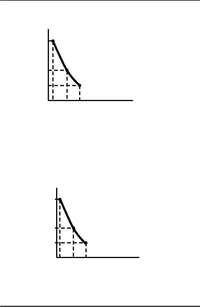
Effect
of a Price Change
Price
of
Food
Individual
Demand relates
E
the
quantity of a good
that
$2.00
a
consumer will buy to
the
price
of that good.
G
$1.00
Demand
Curve
$.50
H
Food
(units
4
12
20
per
month)
Individual
Demand
The
Individual Demand
Curve
Two
Important Properties of Demand
Curves
1) The
level of utility that can be
attained changes as we move
along the curve.
2) At every
point on the demand curve,
the consumer is maximizing
utility by satisfying
the
condition that the MRS
of
food for clothing equals
the ratio of the prices of
food and
clothing.
Effect
of a Price Change
When
the price falls:
Pf /Pc &
MRS also fall
Price
of
Food
E
$2.00
�E: P /P = 2/2 = 1 =
MRS
f
c
�G: P /P = 1/2 = .5 =
MRS
G
$1.00
f
c
�H:P /P = .5/2 = .25 =
MRS
Demand
Curve
f
c
$.50
H
Food
(units
12
4
20
per
month)
Individual
Demand
Income
Changes
Using the
figures developed in the
previous chapter, the impact
of a change in the
income
can be illustrated using
indifference curves.
48
Microeconomics
ECO402
VU
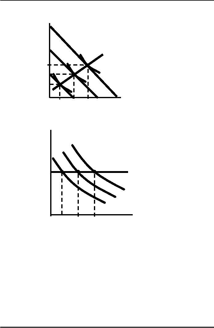
Effects
of Income Changes
Clothing
Assume:
Pf =
$1
(units
per
Pc = $2
month)
I
= $10,
$20,
$30
Income-Consumption
Curve
7
D
An
increase in income,
U3
with
the prices fixed,
5
U2
causes
consumers to alter
B
their
choice of
3
U1
market
basket.
A
Food
(units
per
month)
16
10
4
Effects
of Income Changes
Price
An
increase in income,
of
from
$10 to $20 to $30,
food
with
the prices fixed,
shifts
the consumer's
demand
curve to the right.
E
H
G
$100
D3
D2
D1
Food
(units
10
4
16
per
month)
The
income-consumption curve traces
out the utility-maximizing
combinations of food
and
clothing associated with
every income level.
An increase in
income shifts the budget
line to the right,
increasing consumption
along
the
income-consumption curve.
Simultaneously,
the increase in income
shifts the demand curve to
the right.
Normal
Good vs. Inferior
Good
Income
Changes
�
When the
income-consumption curve has a
positive slope:
The quantity demanded
increases with
income.
The income elasticity of
demand is positive.
The good is a
normal
good.
�
When the
income-consumption curve has a
negative slope:
49
Microeconomics
ECO402
VU
The quantity demanded
decreases with
income.
The income elasticity of
demand is negative.
The good is an
inferior
good.
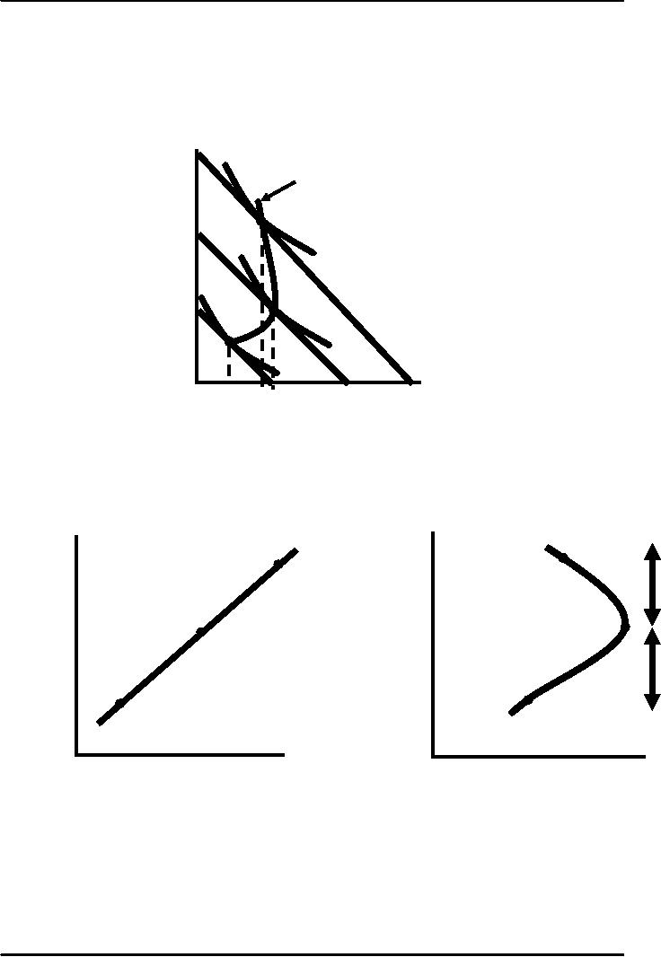
An
Inferior Good
Coffee
15
(units
per
Income-Consumption
month)
Curve
Both
Tea
and
Coffee behave
C
as
a normal good,
between
A and
B...
10
U3
...but
Tea
becomes
an inferior
good
when the income
B
5
consumption
curve
bends
backward
between
B and
C.
U2
A
U1
Tea
30
(units per
month)
5
10
20
Engel
Curves
Engel
Curves
Engel curves relate
the quantity of good
consumed to income.
If the good is a normal
good, the Engel curve is
upward sloping.
If the good is an inferior
good, the Engel curve is
downward sloping.
Income
Income
($
per
30
30
($
per
month)
month)
Inferior
Engel
curves slope
Engel
curves
backward
bending
slope
20
20
for
inferior goods.
upward
for
normal
goods.
Normal
10
10
Food
(units
Food
(units
per
month)
0
16
4
8
12
per
month)
0
16
4
8
12
50

Microeconomics
ECO402
VU
Consumer
Expenditures in US
Income
Group (1997 $)
Expenditure
Less
than 1,000- 20,000- 30,000-
40,000- 50,000-
70,000-
($)
on
$10,000
19,000 29,000 39,000 49,000
69,000 and
above
Entertainment
700
947
1274
1514
2054
2654
4300
Owned
Res.
1116
1725
253
3243
4454
5793
9898
Rented
Res.
1957
2170
2371
2536
2137
1540
1266
Health
Care
1031
1697
1918
820
2052
2214
2642
Food
656
3385
4109
4888
5429
6220
8279
Clothing
859
978
1363
1772
1778
2614
3442
Individual
Demand
Substitutes
and Complements
1)
Two goods are considered
substitutes
if
an increase (decrease) in the
price of one leads to
an
increase (decrease) in the
quantity demanded of the
other.
�e.g. movie tickets
and video rentals
2)
Two goods are considered
complements
if
an increase (decrease) in the
price of one leads
to
a decrease (increase) in the
quantity demanded of the
other.
�e.g. gasoline and
motor oil
3)
Two goods are independent
when a change in the price
of one good has no effect on
the
quantity
demanded of the other
If the price consumption
curve is downward-sloping, the
two goods are
considered
substitutes.
If the price consumption
curve is upward-sloping, the
two goods are
considered
complements.
They
could be both!
51
Table of Contents:
- ECONOMICS:Themes of Microeconomics, Theories and Models
- Economics: Another Perspective, Factors of Production
- REAL VERSUS NOMINAL PRICES:SUPPLY AND DEMAND, The Demand Curve
- Changes in Market Equilibrium:Market for College Education
- Elasticities of supply and demand:The Demand for Gasoline
- Consumer Behavior:Consumer Preferences, Indifference curves
- CONSUMER PREFERENCES:Budget Constraints, Consumer Choice
- Note it is repeated:Consumer Preferences, Revealed Preferences
- MARGINAL UTILITY AND CONSUMER CHOICE:COST-OF-LIVING INDEXES
- Review of Consumer Equilibrium:INDIVIDUAL DEMAND, An Inferior Good
- Income & Substitution Effects:Determining the Market Demand Curve
- The Aggregate Demand For Wheat:NETWORK EXTERNALITIES
- Describing Risk:Unequal Probability Outcomes
- PREFERENCES TOWARD RISK:Risk Premium, Indifference Curve
- PREFERENCES TOWARD RISK:Reducing Risk, The Demand for Risky Assets
- The Technology of Production:Production Function for Food
- Production with Two Variable Inputs:Returns to Scale
- Measuring Cost: Which Costs Matter?:Cost in the Short Run
- A Firm’s Short-Run Costs ($):The Effect of Effluent Fees on Firms’ Input Choices
- Cost in the Long Run:Long-Run Cost with Economies & Diseconomies of Scale
- Production with Two Outputs--Economies of Scope:Cubic Cost Function
- Perfectly Competitive Markets:Choosing Output in Short Run
- A Competitive Firm Incurring Losses:Industry Supply in Short Run
- Elasticity of Market Supply:Producer Surplus for a Market
- Elasticity of Market Supply:Long-Run Competitive Equilibrium
- Elasticity of Market Supply:The Industry’s Long-Run Supply Curve
- Elasticity of Market Supply:Welfare loss if price is held below market-clearing level
- Price Supports:Supply Restrictions, Import Quotas and Tariffs
- The Sugar Quota:The Impact of a Tax or Subsidy, Subsidy
- Perfect Competition:Total, Marginal, and Average Revenue
- Perfect Competition:Effect of Excise Tax on Monopolist
- Monopoly:Elasticity of Demand and Price Markup, Sources of Monopoly Power
- The Social Costs of Monopoly Power:Price Regulation, Monopsony
- Monopsony Power:Pricing With Market Power, Capturing Consumer Surplus
- Monopsony Power:THE ECONOMICS OF COUPONS AND REBATES
- Airline Fares:Elasticities of Demand for Air Travel, The Two-Part Tariff
- Bundling:Consumption Decisions When Products are Bundled
- Bundling:Mixed Versus Pure Bundling, Effects of Advertising
- MONOPOLISTIC COMPETITION:Monopolistic Competition in the Market for Colas and Coffee
- OLIGOPOLY:Duopoly Example, Price Competition
- Competition Versus Collusion:The Prisoners’ Dilemma, Implications of the Prisoners
- COMPETITIVE FACTOR MARKETS:Marginal Revenue Product
- Competitive Factor Markets:The Demand for Jet Fuel
- Equilibrium in a Competitive Factor Market:Labor Market Equilibrium
- Factor Markets with Monopoly Power:Monopoly Power of Sellers of Labor