 |
CONSUMPTION:Secular Stagnation and Simon Kuznets |
| << GOVERNMENT DEBT (Continued…):Starting with too little capital, |
| CONSUMPTION (Continued…):Consumer Preferences, Constraints on Borrowings >> |

Macroeconomics
ECO 403
VU
LESSON
37
CONSUMPTION
John
Maynard Keynes and the
Consumption Function
The
consumption function was
central to Keynes' theory of
economic fluctuations presented
in
The
General Theory in
1936.
�
Keynes
conjectured that the
marginal
propensity to consume-- the
amount
consumed
out of an additional dollar of
income-- is between zero and
one. He claimed
that
the fundamental law is that
out of every dollar of
earned income, people
will
consume
part of it and save the
rest.
�
Keynes
also proposed the average
propensity to consume-- the
ratio of consumption
to
income-- falls as income
rises.
�
Keynes
also held that income is
the primary determinant of
consumption and that
the
interest
rate does not have an
important role.
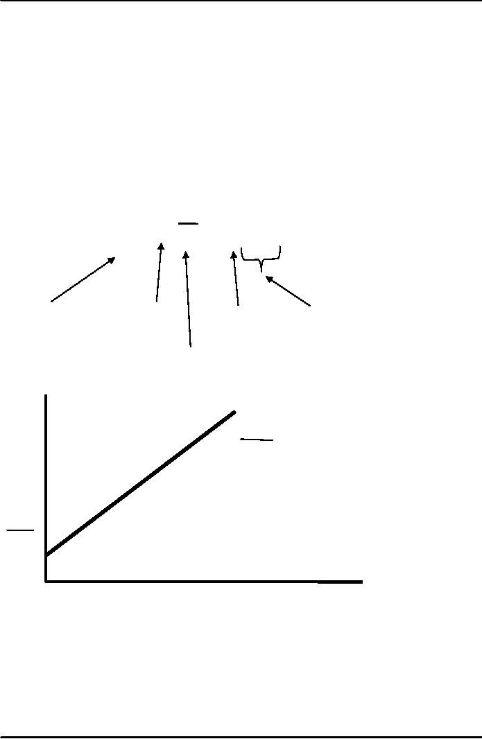
The
Consumption Function
C
= C + cY
income
depends
Marginal
consumption
on
Propensity
to
spending
by
consume
(MPC)
households
Autonomous
consumption
C
C
= C + cY
C
Y
This
consumption function exhibits
three properties that Keynes
conjectured.
1.
The marginal propensity to
consume c is between zero
and one.
2.
The average propensity to
consume falls as income
rises.
3.
Consumption is determined by current
income.
173

Macroeconomics
ECO 403
VU
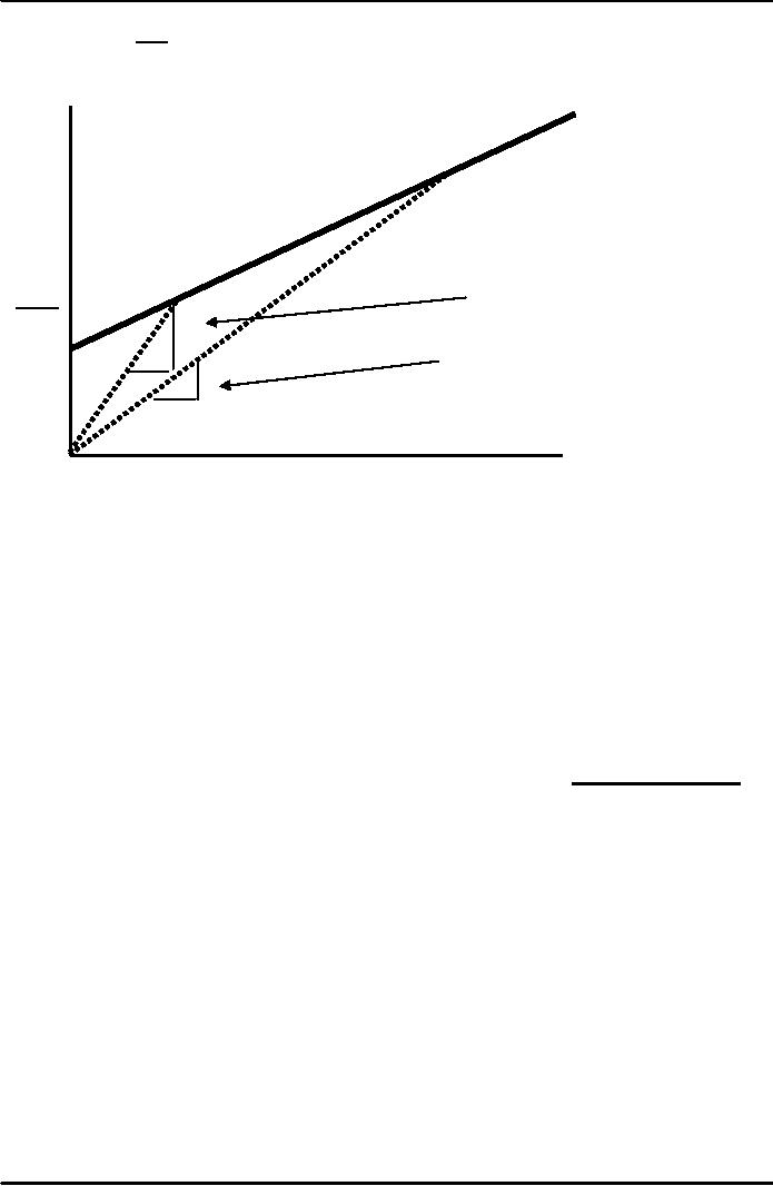
Average
Propensity to Consume
APC
= C/Y = C/Y + c
As
Y rises, C/Y falls, and so
the average propensity to
consume C/Y falls. Notice
that the
interest
rate is not included in this
function.
C
APC1
C
APC2
1
1
Y
Marginal
Propensity to Consume
�
To
understand the marginal
propensity to consume (MPC),
consider a shopping
scenario.
A
person who loves to shop
probably has a large MPC,
let's say (.99).
This
means
that for every extra
rupee
he or she earns after tax
deductions, he or
she
spends 99 paisas of
it.
�
The MPC
measures the sensitivity of
the change in one variable
(C) with respect to a
change
in the other variable
(Y).
Secular
Stagnation and Simon
Kuznets
�
During
World War II, on the
basis of Keynes' consumption
function, economists
predicted
that the economy would
experience what they called
secular
stagnation, a
long
depression of infinite duration--
unless fiscal policy was
used to stimulate
aggregate
demand.
�
It
turned out that the
end of the war did
not throw the U.S.
into another depression,
but
it
did suggest that Keynes'
conjecture that the average
propensity to consume
would
fall
as income rose appeared not
to hold.
�
Simon
Kuznets constructed new
aggregate data on consumption
and investment
dating
back to 1869 and whose
work would later earn a
Nobel Prize.
�
He
discovered that the ratio of
consumption to income was
stable over time,
despite
large
increases in income; again,
Keynes' conjecture was
called into question.
�
This
brings us to the
puzzle...
Consumption
Puzzle
�
The
failure of the secular-stagnation
hypothesis and the findings
of Kuznets both
indicated
that
the average propensity to
consume is fairly constant
over time. This presented
a
puzzle:
why did Keynes' conjectures
hold up well in the studies
of household data and
in
the
studies of short time-series,
but fail when long
time series were
examined?
174

Macroeconomics
ECO 403
VU
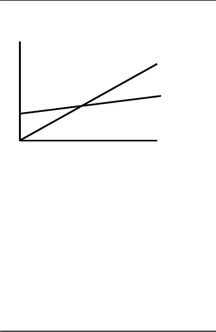
Studies
of household data and short
time-series found a relationship
between consumption
and
income similar to the one
Keynes conjectured-- this is
called the short-run
consumption
function.
But,
studies using long
time-series found that the
APC did not vary
systematically with
income-
-this
relationship is called the
long-run consumption
function.
C
Long-run
consumption function
(constant
APC)
Short-run
consumption
function
(falling APC)
Y
Irving
Fisher and Intertemporal
Choice
�
The
economist Irving Fisher
developed the model with
which economists analyze
how
rational,
forward-looking consumers make
intertemporal choices-- that
is, choices
involving
different periods of
time.
�
The
model illuminates
the
constraints consumers
face,
�
the
preferences they have,
and
�
how
these constraints and
preferences together determine
their choices about
�
consumption
and saving.
When
consumers are deciding how
much to consume today versus
how much to consume
in
the
future, they face an intertemporal
budget constraint, which
measures the total
resources
available
for consumption today and in
the future.
Consumer's
Budget Constraint
�
Consider
the decision facing a
consumer who lives for
two periods (representing
youth &
age)
�
He
earns Income Y1,
Y2 and consumes C1,
C2 in both periods
respectively (adjusted
for
inflation)
�
The
savings in the first period
will be
S
= Y1
C1
�
In
the second period
175

Macroeconomics
ECO 403
VU
C2 = (1 + r) S +
Y2
Where
r is the real interest
rate.
�
Remember
S can represent either
saving or borrowing and the
equations hold in
both
cases.
If C1 <
Y1
consumer
is saving
S>0
If C1 >
Y1
consumer
is borrowing
S<0
�
Assume:
r
(borrowing) = r (saving)
Combining
the two equations:
C2 = (1 +
r)(Y1
C1) +
Y2
Rearranging
(1
+ r)C1 +
C2 = (1 + r) Y1 + Y2
�
Dividing
both sides by 1 + r
C2
Y2
C1
+
r
+
1+r
=
Y1 +
1
So
we can say that
�
The
consumer's budget constraint
implies that if the interest
rate is zero, the
budget
constraint
shows that total consumption
in the two periods equals
total income in the
two
periods. In the usual case
in which the interest rate
is greater than zero,
future
consumption
and future income are
discounted by a factor of 1 + r.
�
This
discounting
arises
from the interest earned on
savings. Because the
consumer
earns
interest on current income
that is saved, future income
is worth less than
current
income.
�
Also,
because future consumption is
paid for out of savings
that have earned
interest,
future
consumption costs less than
current consumption.
The
factor 1/(1+r) is the price
of second-period consumption measured in
terms of first-
�
period
consumption; it is the amount of
first-period consumption that
the consumer
must
forgo to obtain 1 unit of
second-period consumption.
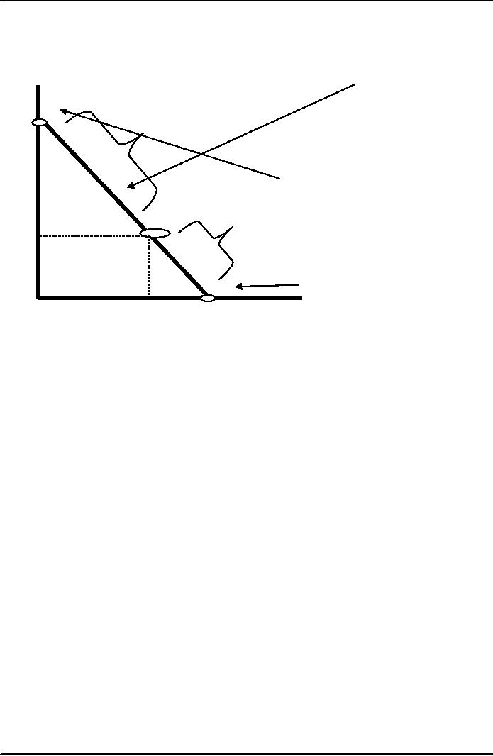
Here
are the combinations of
first-period and second-period
consumption the consumer
can
choose.
176

Macroeconomics
ECO 403
VU
Second-
period
consumption
Consumer's
budget
constraint
B
Saving
Vertical
intercept is
(1+r)Y1 +
Y2
A
Borrowing
Y2
Horizontal
intercept is
C
Y1 +
Y2/(1+r)
Y1
First-period
consumption
If
he chooses a point between A
and B, he consumes less than
his income in the first
period
and
saves the rest for
the second period. If he
chooses between A and C, he
consumes more
that
his income in the first
period and borrows to make
up the difference.
177
Table of Contents:
- INTRODUCTION:COURSE DESCRIPTION, TEN PRINCIPLES OF ECONOMICS
- PRINCIPLE OF MACROECONOMICS:People Face Tradeoffs
- IMPORTANCE OF MACROECONOMICS:Interest rates and rental payments
- THE DATA OF MACROECONOMICS:Rules for computing GDP
- THE DATA OF MACROECONOMICS (Continued…):Components of Expenditures
- THE DATA OF MACROECONOMICS (Continued…):How to construct the CPI
- NATIONAL INCOME: WHERE IT COMES FROM AND WHERE IT GOES
- NATIONAL INCOME: WHERE IT COMES FROM AND WHERE IT GOES (Continued…)
- NATIONAL INCOME: WHERE IT COMES FROM AND WHERE IT GOES (Continued…)
- NATIONAL INCOME: WHERE IT COMES FROM AND WHERE IT GOES (Continued…)
- MONEY AND INFLATION:The Quantity Equation, Inflation and interest rates
- MONEY AND INFLATION (Continued…):Money demand and the nominal interest rate
- MONEY AND INFLATION (Continued…):Costs of expected inflation:
- MONEY AND INFLATION (Continued…):The Classical Dichotomy
- OPEN ECONOMY:Three experiments, The nominal exchange rate
- OPEN ECONOMY (Continued…):The Determinants of the Nominal Exchange Rate
- OPEN ECONOMY (Continued…):A first model of the natural rate
- ISSUES IN UNEMPLOYMENT:Public Policy and Job Search
- ECONOMIC GROWTH:THE SOLOW MODEL, Saving and investment
- ECONOMIC GROWTH (Continued…):The Steady State
- ECONOMIC GROWTH (Continued…):The Golden Rule Capital Stock
- ECONOMIC GROWTH (Continued…):The Golden Rule, Policies to promote growth
- ECONOMIC GROWTH (Continued…):Possible problems with industrial policy
- AGGREGATE DEMAND AND AGGREGATE SUPPLY:When prices are sticky
- AGGREGATE DEMAND AND AGGREGATE SUPPLY (Continued…):
- AGGREGATE DEMAND AND AGGREGATE SUPPLY (Continued…):
- AGGREGATE DEMAND AND AGGREGATE SUPPLY (Continued…)
- AGGREGATE DEMAND AND AGGREGATE SUPPLY (Continued…)
- AGGREGATE DEMAND AND AGGREGATE SUPPLY (Continued…)
- AGGREGATE DEMAND IN THE OPEN ECONOMY:Lessons about fiscal policy
- AGGREGATE DEMAND IN THE OPEN ECONOMY(Continued…):Fixed exchange rates
- AGGREGATE DEMAND IN THE OPEN ECONOMY (Continued…):Why income might not rise
- AGGREGATE SUPPLY:The sticky-price model
- AGGREGATE SUPPLY (Continued…):Deriving the Phillips Curve from SRAS
- GOVERNMENT DEBT:Permanent Debt, Floating Debt, Unfunded Debts
- GOVERNMENT DEBT (Continued…):Starting with too little capital,
- CONSUMPTION:Secular Stagnation and Simon Kuznets
- CONSUMPTION (Continued…):Consumer Preferences, Constraints on Borrowings
- CONSUMPTION (Continued…):The Life-cycle Consumption Function
- INVESTMENT:The Rental Price of Capital, The Cost of Capital
- INVESTMENT (Continued…):The Determinants of Investment
- INVESTMENT (Continued…):Financing Constraints, Residential Investment
- INVESTMENT (Continued…):Inventories and the Real Interest Rate
- MONEY:Money Supply, Fractional Reserve Banking,
- MONEY (Continued…):Three Instruments of Money Supply, Money Demand