 |
Macroeconomics
ECO 403
VU
LESSON
31
AGGREGATE
DEMAND IN THE OPEN
ECONOMY(Continued...)
Equilibrium
in the Mundell-Fleming
model
Y
= C
(Y
- T
) +
I
(r
*) +
G
+ NX
(e
)
M
P = L
(r
*,Y
)
LM*
e
equilibrium
exchange
rate
IS*
equilibrium
Y
level
of
income
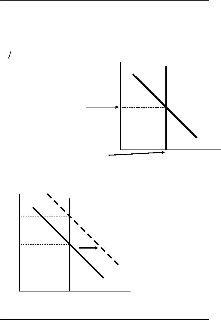
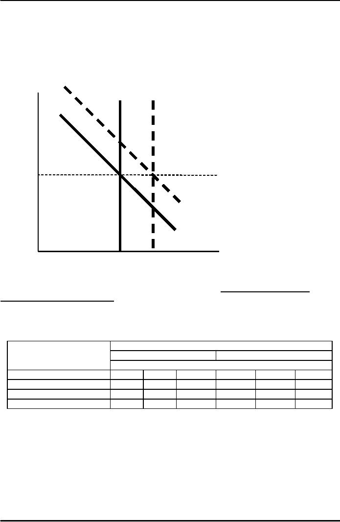
Fiscal
policy under floating
exchange rates
At
any given value of e, a
fiscal expansion increases Y,
shifting IS* to the right.
Results: Δe >
0,
ΔY
= 0
LM*1
e
e2
e1
IS*2
IS*1
Y
Y1
Results: Δe >
0, ΔY =
0
145
Macroeconomics
ECO 403
VU
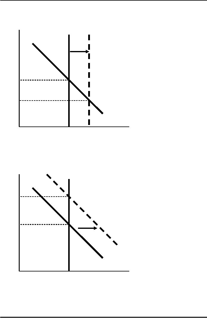
Monetary
policy under floating
exchange rates
An
increase in M shifts LM*
right because Y must rise to
restore equilibrium in the
money
market.
e
LM*1
LM*2
e1
e2
IS*1
Y
Y1
Y2
Results:
Δe <
0, ΔY >
0
Trade
policy under floating
exchange rates
At
any given value of e, a
tariff or quota reduces
imports, increases NX, and
shifts IS* to the
right.
LM*1
e
e2
e1
IS*2
IS*1
Y
Y1
Lessons
about trade
policy
�
Import
restrictions cannot reduce a
trade deficit.
�
Even
though NX is unchanged, there is
less trade:
146
Macroeconomics
ECO 403
VU
The trade
restriction reduces
imports
Exchange
rate appreciation reduces
exports
Less
trade means fewer `gains
from trade.'
�
Import
restrictions on specific products
save jobs in the domestic
industries that
produce
those
products, but destroy jobs
in export-producing sectors.
Hence,
import restrictions fail to
increase total
employment.
Worse
yet, import restrictions
create "sectoral shifts,"
which cause
frictional
unemployment.
Fixed
exchange rates
�
Under
a system of fixed exchange
rates, the country's central
bank stands ready to buy
or
sell
the domestic currency for
foreign currency at a predetermined
rate.
�
In
the context of the
Mundell-Fleming model, the
central bank shifts the LM*
curve as
required
to keep e at its pre-announced
rate.
�
This
system fixes the nominal
exchange rate.
In
the long run, when
prices are flexible, the
real exchange rate can
move even if the
nominal
rate is fixed.
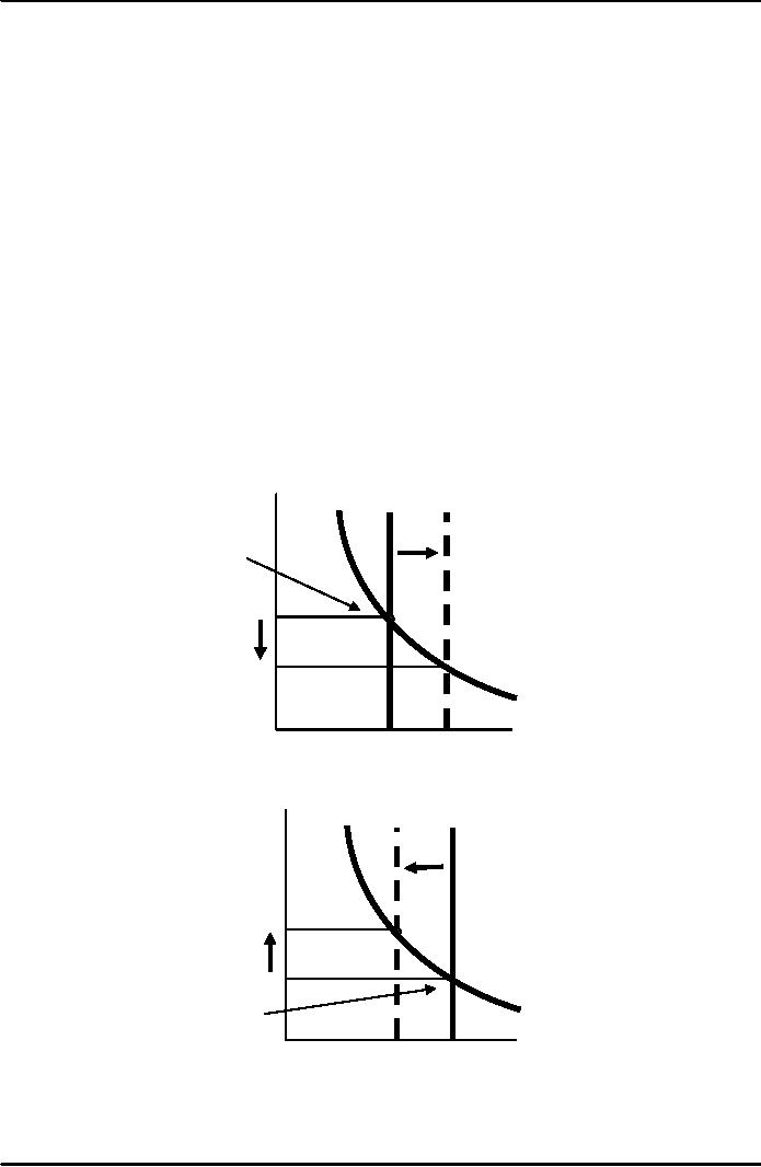
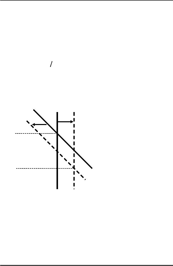
a.
The Equilibrium exchange
rate is Greater than the
fixed exchange rate
LM1 LM2
e
Equilibrium
exchange
rate
>
>
>
Fixed
exchange rate
IS*
Income,
Output, Y
b.
The Equilibrium exchange
rate is less than the
fixed exchange rate
LM2 LM1
e
Fixed
exchange rate
>
>>
IS*
Equilibrium
exchange rate
Income,
Output, Y
147
Macroeconomics
ECO 403
VU
Fiscal
policy under fixed exchange
rates
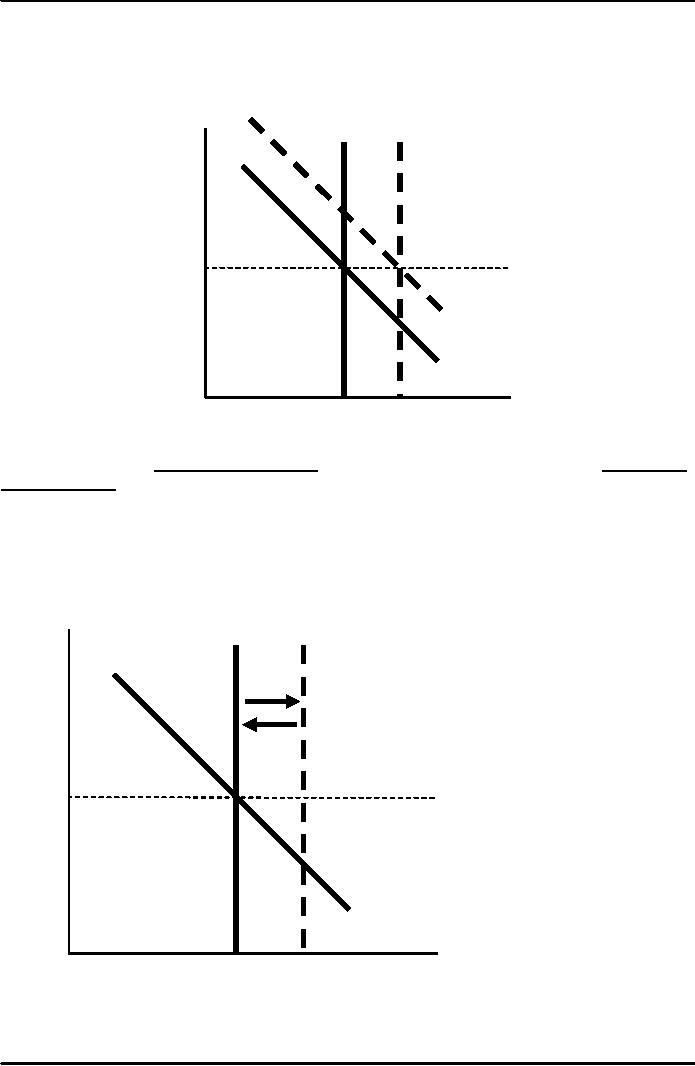
Under
fixed exchange rates, a
fiscal expansion would raise
e. To keep e from
rising,
the
central bank must sell
domestic currency, which
increases M and shifts LM*
right.
LM*1
LM*2
e
e1
IS*2
IS*1
Y
Y1
Y2
Results:
Δe =
0, ΔY >
0
Under
floating rates, fiscal
policy ineffective at changing
output. Under fixed rates,
fiscal policy
is
very effective at changing
output. LM
shifts out!
Monetary
policy under fixed exchange
rates
An
increase in M would shift LM*
right and reduce e. To
prevent the fall in e, the
central bank
must
buy domestic currency, which
reduces M and shifts LM*
back left.
LM*1
LM*2
e
e1
IS*1
Y
Y1
Y2
Results:
Δe =
0, ΔY =
0
148
Macroeconomics
ECO 403
VU
Under
floating rates, monetary
policy is very effective at
changing output. Under fixed
rates,
monetary
policy cannot be used to
affect output.
Trade
policy under fixed exchange
rates
A
restriction on imports puts
upward pressure on e.
To keep e
from
rising, the central
bank
must
sell domestic currency,
which increases M
and
shifts LM*
right.
LM*1
LM*2
e
e1
IS*2
IS*1
Y
Y1
Y2
Results:
Δe =
0, ΔY >
0
Under
floating rates, import
restrictions do not affect Y or NX.
Under fixed rates,
import
restrictions
increase Y and NX. But,
these gains come at the
expense of other countries,
as
the
policy merely shifts demand
from foreign to domestic
goods
M-F:
summary of policy
effects
Type
of Exchange Rate
Regime
Floating
Fixed
Impact
on
Policy
Y
e
NX
Y
e
NX
Fiscal
Expansion
0
0
0
Monetary
Expansion
0
0
0
Import
Restriction
0
0
0
Interest-rate
differentials
Two
reasons why r may differ
from r*
�
Country
risk:
The
risk that the country's
borrowers will default on
their loan repayments
because of
political
or economic turmoil. Lenders
require a higher interest
rate to compensate
them
for this risk.
149
Macroeconomics
ECO 403
VU
�
Expected
exchange rate
changes:
If
a country's exchange rate is
expected to fall, then its
borrowers must pay a
higher
interest
rate to compensate lenders
for the expected currency
depreciation.
Differentials
in the M-F model
r
= r
*+ θ
Where
θ
is a
risk premium.
Substitute
the expression for r into
the IS* and LM*
equations:
Y
= C
(Y
- T
) +
I
(r
* + θ )
+
G
+ NX
(e
)
M
P = L
(r
* + θ ,Y
)
The
effects of an increase in θ
IS*
shifts left, because ↑
θ ⇒ ↑r
⇒
↓I
LM*
shifts
right, because ↑
θ ⇒
↑r
⇒
↓(M/P) d,
So
Y must rise to restore money
market equilibrium.
LM*1
LM*2
e1
e2
IS*1
IS*2
Y1
Y2
The
effects of an increase in θ
�
The
fall in e is intuitive:
An
increase in country risk or an
expected depreciation makes
holding the country's
currency
less attractive.
Note:
an expected depreciation is a
self-fulfilling prophecy.
�
The
increase in Y occurs because
the boost in NX (from the
depreciation) is even
greater
than
the fall in I (from the
rise in r).
150
Table of Contents:
- INTRODUCTION:COURSE DESCRIPTION, TEN PRINCIPLES OF ECONOMICS
- PRINCIPLE OF MACROECONOMICS:People Face Tradeoffs
- IMPORTANCE OF MACROECONOMICS:Interest rates and rental payments
- THE DATA OF MACROECONOMICS:Rules for computing GDP
- THE DATA OF MACROECONOMICS (Continued…):Components of Expenditures
- THE DATA OF MACROECONOMICS (Continued…):How to construct the CPI
- NATIONAL INCOME: WHERE IT COMES FROM AND WHERE IT GOES
- NATIONAL INCOME: WHERE IT COMES FROM AND WHERE IT GOES (Continued…)
- NATIONAL INCOME: WHERE IT COMES FROM AND WHERE IT GOES (Continued…)
- NATIONAL INCOME: WHERE IT COMES FROM AND WHERE IT GOES (Continued…)
- MONEY AND INFLATION:The Quantity Equation, Inflation and interest rates
- MONEY AND INFLATION (Continued…):Money demand and the nominal interest rate
- MONEY AND INFLATION (Continued…):Costs of expected inflation:
- MONEY AND INFLATION (Continued…):The Classical Dichotomy
- OPEN ECONOMY:Three experiments, The nominal exchange rate
- OPEN ECONOMY (Continued…):The Determinants of the Nominal Exchange Rate
- OPEN ECONOMY (Continued…):A first model of the natural rate
- ISSUES IN UNEMPLOYMENT:Public Policy and Job Search
- ECONOMIC GROWTH:THE SOLOW MODEL, Saving and investment
- ECONOMIC GROWTH (Continued…):The Steady State
- ECONOMIC GROWTH (Continued…):The Golden Rule Capital Stock
- ECONOMIC GROWTH (Continued…):The Golden Rule, Policies to promote growth
- ECONOMIC GROWTH (Continued…):Possible problems with industrial policy
- AGGREGATE DEMAND AND AGGREGATE SUPPLY:When prices are sticky
- AGGREGATE DEMAND AND AGGREGATE SUPPLY (Continued…):
- AGGREGATE DEMAND AND AGGREGATE SUPPLY (Continued…):
- AGGREGATE DEMAND AND AGGREGATE SUPPLY (Continued…)
- AGGREGATE DEMAND AND AGGREGATE SUPPLY (Continued…)
- AGGREGATE DEMAND AND AGGREGATE SUPPLY (Continued…)
- AGGREGATE DEMAND IN THE OPEN ECONOMY:Lessons about fiscal policy
- AGGREGATE DEMAND IN THE OPEN ECONOMY(Continued…):Fixed exchange rates
- AGGREGATE DEMAND IN THE OPEN ECONOMY (Continued…):Why income might not rise
- AGGREGATE SUPPLY:The sticky-price model
- AGGREGATE SUPPLY (Continued…):Deriving the Phillips Curve from SRAS
- GOVERNMENT DEBT:Permanent Debt, Floating Debt, Unfunded Debts
- GOVERNMENT DEBT (Continued…):Starting with too little capital,
- CONSUMPTION:Secular Stagnation and Simon Kuznets
- CONSUMPTION (Continued…):Consumer Preferences, Constraints on Borrowings
- CONSUMPTION (Continued…):The Life-cycle Consumption Function
- INVESTMENT:The Rental Price of Capital, The Cost of Capital
- INVESTMENT (Continued…):The Determinants of Investment
- INVESTMENT (Continued…):Financing Constraints, Residential Investment
- INVESTMENT (Continued…):Inventories and the Real Interest Rate
- MONEY:Money Supply, Fractional Reserve Banking,
- MONEY (Continued…):Three Instruments of Money Supply, Money Demand