 |
AGGREGATE DEMAND AND AGGREGATE SUPPLY (Continued…) |
| << AGGREGATE DEMAND AND AGGREGATE SUPPLY (Continued…) |
| AGGREGATE DEMAND IN THE OPEN ECONOMY:Lessons about fiscal policy >> |
Macroeconomics
ECO 403
VU
LESSON
29
AGGREGATE
DEMAND AND AGGREGATE SUPPLY
(Continued...)
IS-LM
and Aggregate
Demand
�
So
far, we've been using
the IS-LM
model
to analyze the short run,
when the price
level
is assumed fixed.
�
However, a
change in P would shift the
LM curve
and therefore affect
Y.
�
The
aggregate demand curve
captures this relationship
between P and Y
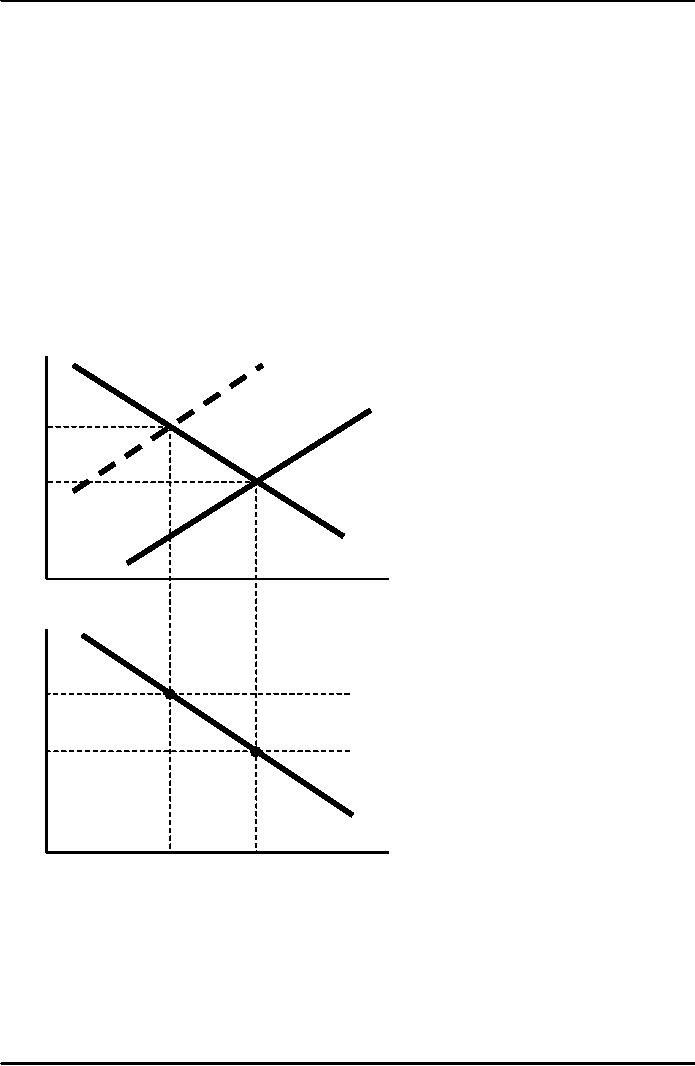
Deriving
the AD
curve
Intuition
for slope of AD
curve:
↑P
⇒
↓(M/P)
⇒
LM shifts
left
⇒
↑r
⇒
↓I
⇒
↓Y
LM(P2)
r
LM(P1)
r2
r1
IS
Y1
Y
Y2
P
P2
P1
AD
Y
Y2
Y1
Monetary
policy and the AD
curve
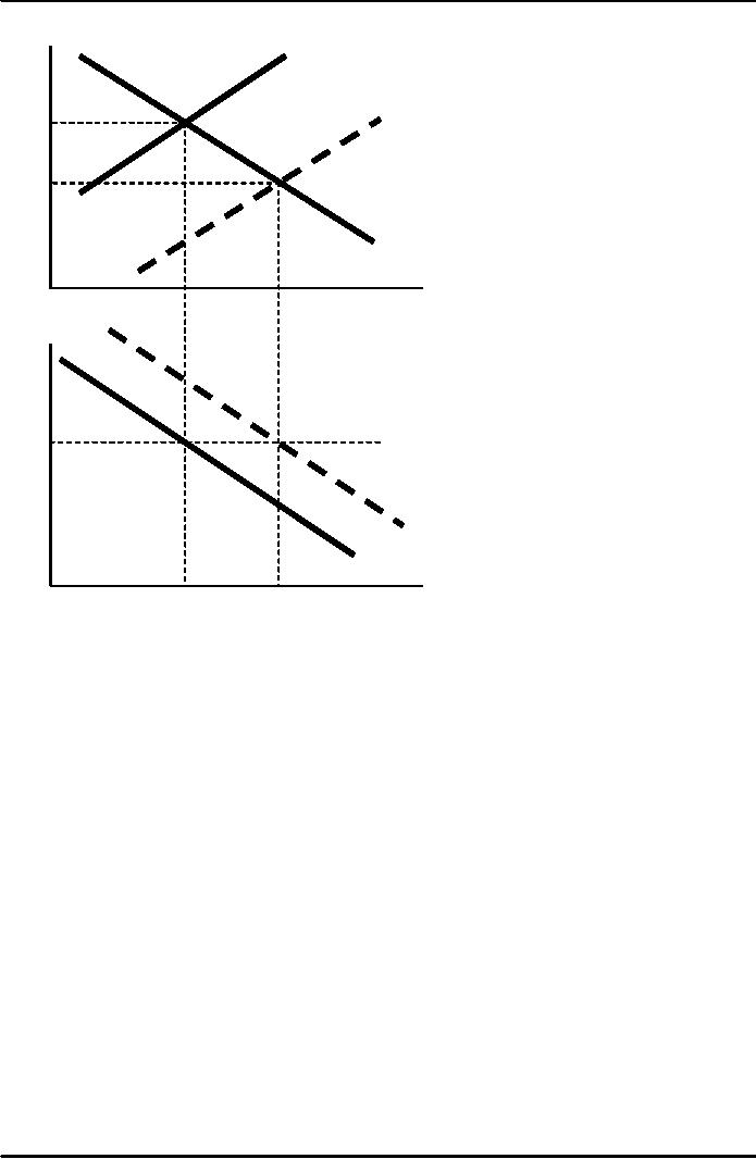
The
central bank can increase
aggregate demand:
↑M ⇒
LM shifts
right
⇒
↓r
⇒
↑I
⇒
↑Y at
each value of P
132
Macroeconomics
ECO 403
VU
LM(M1/P1)
r
LM(M2/P1)
r1
r2
IS
Y2
Y
Y1
P
P1
AD2
AD1
Y
Y1
Y2
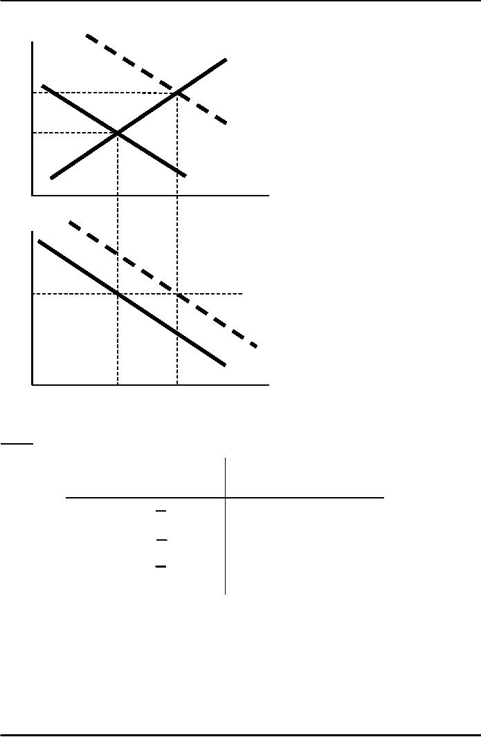
Fiscal
policy and the AD
curve
Expansionary
fiscal policy (↑G and/or
↓T)
increases aggregate
demand:
↓T ⇒
↑C
⇒
IS
shifts right
⇒
↑Y at
each value of P
133
Macroeconomics
ECO 403
VU
r
LM
r2
r1
IS2
IS1
Y2
Y
Y1
P
P1
AD2
AD1
Y
Y2
Y1
IS-LM
and
AD-AS
in
the short run & long
run
Recall:
The
force that moves the
economy from the short
run to the long run is
the gradual
adjustment
of prices.
In
the short-run
equilibrium,
then
over time, the
price
if
level
will
Y>Y
Rise
Y<Y
Fall
Y=Y
remain
constant
134
Macroeconomics
ECO 403
VU
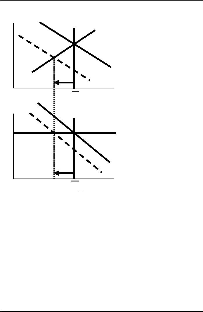
The
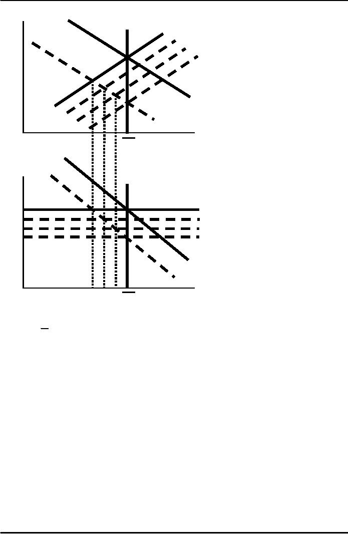
SR and LR effects of an IS
shock
A
negative IS shock shifts IS
and AD left, causing Y to
fall.
LRAS
r
LM(P1)
IS1
IS2
Y
Y
P
LRAS
SRAS1
P1
AD1
AD2
Y
Y
In
the new short-run
equilibrium, Y < Y.
Over
time, P gradually falls,
which causes
�
SRAS
to
move down
�
M/P to
increase, which causes
LM to
move down
135
Macroeconomics
ECO 403
VU
r
LRAS
LM(P2)
IS1
IS2
Y
Y
P
LRAS
SRAS1
P1
SRAS2
P2
AD1
AD2
Y
Y
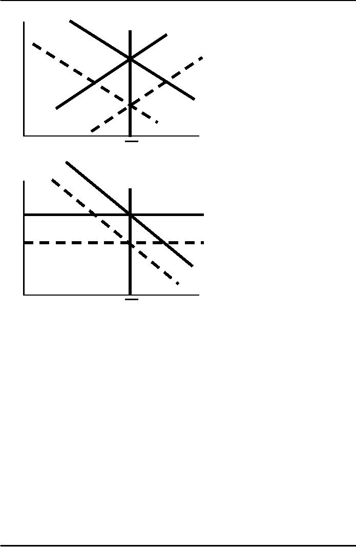
This
process continues until
economy reaches a long-run
equilibrium with Y = Y.
136
Macroeconomics
ECO 403
VU
r
LRAS
LM(P1)
LM(P2)
IS1
IS2
Y
Y
P
LRAS
SRAS1
P1
SRAS2
P2
AD1
AD2
Y
Y
Short
Run Impacts
Now
it's time to determine the
effects on the variables in
the economy.
Y
+,
because Y moved
P
0,
because prices are sticky in
the SR.
+,
because a +ΔY leads to a
rise in r as IS slides along
the LM curve.
r
+,
because a + ΔY increases
the level of consumption (↑C=C(↑Y-T)).
C
I
, since r increased, the
level of investment
decreased.
Long
Run Impacts
Y
0,
because rising P shifts LM to
left, returning Y to Y* as required by
long-run LRAS.
P
+,
in order to eliminate the
excess demand at P0.
+,
reflecting the leftward
shift in LM due to + ΔP
r
C
0,
since both Y and T are
back to their initial levels
(C=C(Y-T))
, since r has risen
even more due to the +
ΔP.
I
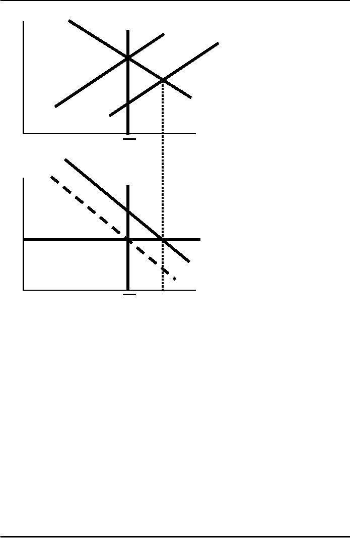
Analyze
SR & LR effects of ΔM
�
We
Have IS-LM and AD-AS
diagrams as shown
here.
�
Suppose
central bank increases
M.
137
Macroeconomics
ECO 403
VU
LM(M1/P1)
r
LRAS
LM(M2/P1)
IS1
Y
Y
P
LRAS
SRAS1
P1
AD2
AD1
Y
Y
138
Macroeconomics
ECO 403
VU
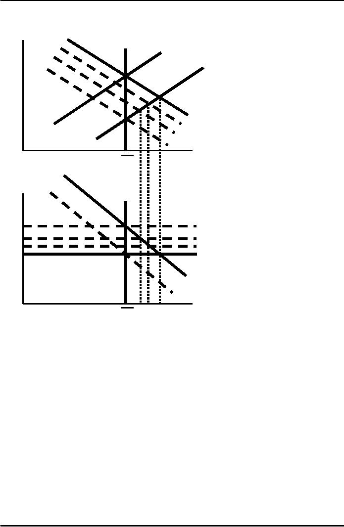
�
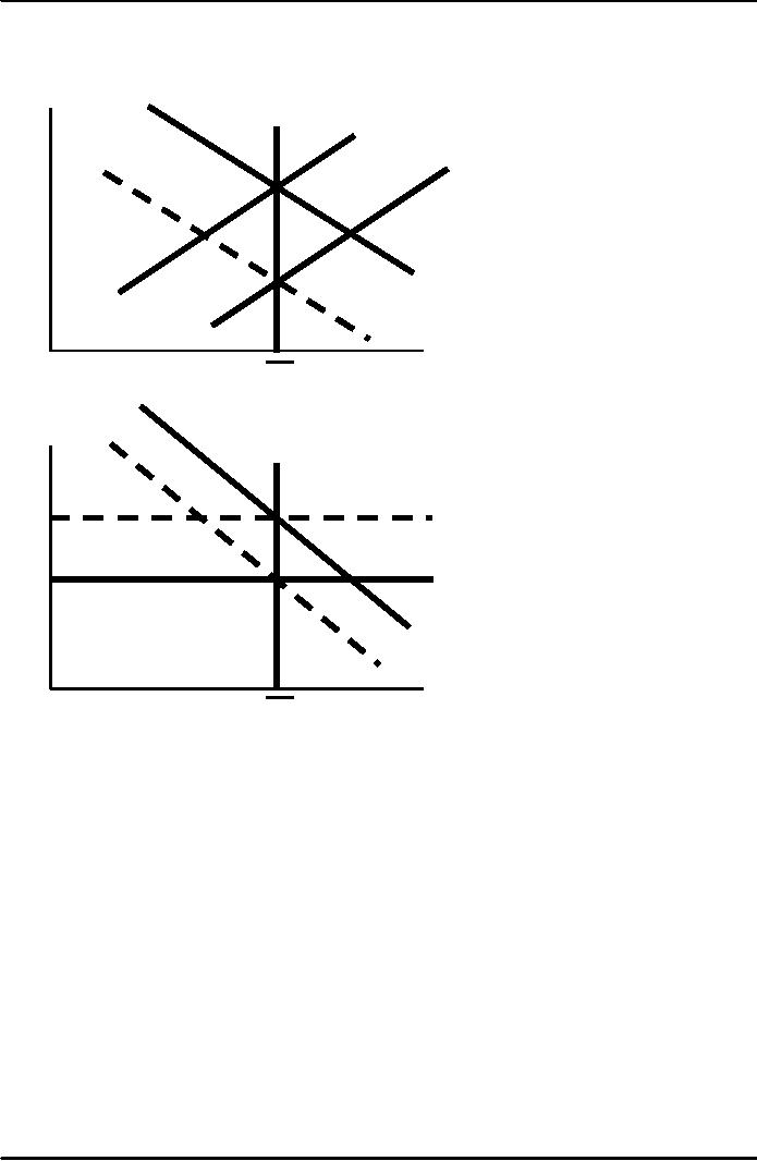
The
Graph below Shows the
Short run effects of the
change in M and what happens
in
the
transition from the short
run to the long
run.
LM(M1/P1)
r
LRAS
LM(M2/P1)
IS1
IS2
Y
Y
P
LRAS
SRAS2
P1
SRAS1
AD2
AD1
Y
Y
139
Macroeconomics
ECO 403
VU
�
The
new long-run equilibrium
values of the endogenous
variables as compared to
their
initial
values
LM(M1/P1)
r
LRAS
LM(M2/P1)
IS1
IS2
Y
Y
P
LRAS
SRAS2
P1
SRAS1
AD2
AD1
Y
Y
Short
Run Impacts
Now
it's time to determine the
effects on the variables in
the economy.
Y
+,
because Y moved
P
0,
because prices are sticky in
the SR.
-,
because a +ΔY leads to a
decrease in r as LM slides along
the IS curve.
r
+,
because a + ΔY increases
the level of consumption (↑C=C(↑Y-T)).
C
I
+
, since r decreased, the
level of investment
increased.
Long
Run Impacts
Y
0,
because rising P shifts LM to
left, returning Y to Y* as required by
long-run LRAS.
P
+,
in order to eliminate the
excess demand at P0.
0,
reflecting the leftward
shift in LM due to + ΔP restoring r to
its original level
r
C
0,
since both Y and T are
back to their initial levels
(C=C(Y-T))
I
0
, since Y or r has not changed.
Notice
that the only LR impact of
an increase in the money
supply was an increase in the
price
level.
140
Table of Contents:
- INTRODUCTION:COURSE DESCRIPTION, TEN PRINCIPLES OF ECONOMICS
- PRINCIPLE OF MACROECONOMICS:People Face Tradeoffs
- IMPORTANCE OF MACROECONOMICS:Interest rates and rental payments
- THE DATA OF MACROECONOMICS:Rules for computing GDP
- THE DATA OF MACROECONOMICS (Continued…):Components of Expenditures
- THE DATA OF MACROECONOMICS (Continued…):How to construct the CPI
- NATIONAL INCOME: WHERE IT COMES FROM AND WHERE IT GOES
- NATIONAL INCOME: WHERE IT COMES FROM AND WHERE IT GOES (Continued…)
- NATIONAL INCOME: WHERE IT COMES FROM AND WHERE IT GOES (Continued…)
- NATIONAL INCOME: WHERE IT COMES FROM AND WHERE IT GOES (Continued…)
- MONEY AND INFLATION:The Quantity Equation, Inflation and interest rates
- MONEY AND INFLATION (Continued…):Money demand and the nominal interest rate
- MONEY AND INFLATION (Continued…):Costs of expected inflation:
- MONEY AND INFLATION (Continued…):The Classical Dichotomy
- OPEN ECONOMY:Three experiments, The nominal exchange rate
- OPEN ECONOMY (Continued…):The Determinants of the Nominal Exchange Rate
- OPEN ECONOMY (Continued…):A first model of the natural rate
- ISSUES IN UNEMPLOYMENT:Public Policy and Job Search
- ECONOMIC GROWTH:THE SOLOW MODEL, Saving and investment
- ECONOMIC GROWTH (Continued…):The Steady State
- ECONOMIC GROWTH (Continued…):The Golden Rule Capital Stock
- ECONOMIC GROWTH (Continued…):The Golden Rule, Policies to promote growth
- ECONOMIC GROWTH (Continued…):Possible problems with industrial policy
- AGGREGATE DEMAND AND AGGREGATE SUPPLY:When prices are sticky
- AGGREGATE DEMAND AND AGGREGATE SUPPLY (Continued…):
- AGGREGATE DEMAND AND AGGREGATE SUPPLY (Continued…):
- AGGREGATE DEMAND AND AGGREGATE SUPPLY (Continued…)
- AGGREGATE DEMAND AND AGGREGATE SUPPLY (Continued…)
- AGGREGATE DEMAND AND AGGREGATE SUPPLY (Continued…)
- AGGREGATE DEMAND IN THE OPEN ECONOMY:Lessons about fiscal policy
- AGGREGATE DEMAND IN THE OPEN ECONOMY(Continued…):Fixed exchange rates
- AGGREGATE DEMAND IN THE OPEN ECONOMY (Continued…):Why income might not rise
- AGGREGATE SUPPLY:The sticky-price model
- AGGREGATE SUPPLY (Continued…):Deriving the Phillips Curve from SRAS
- GOVERNMENT DEBT:Permanent Debt, Floating Debt, Unfunded Debts
- GOVERNMENT DEBT (Continued…):Starting with too little capital,
- CONSUMPTION:Secular Stagnation and Simon Kuznets
- CONSUMPTION (Continued…):Consumer Preferences, Constraints on Borrowings
- CONSUMPTION (Continued…):The Life-cycle Consumption Function
- INVESTMENT:The Rental Price of Capital, The Cost of Capital
- INVESTMENT (Continued…):The Determinants of Investment
- INVESTMENT (Continued…):Financing Constraints, Residential Investment
- INVESTMENT (Continued…):Inventories and the Real Interest Rate
- MONEY:Money Supply, Fractional Reserve Banking,
- MONEY (Continued…):Three Instruments of Money Supply, Money Demand