 |
AGGREGATE DEMAND AND AGGREGATE SUPPLY (Continued…) |
| << AGGREGATE DEMAND AND AGGREGATE SUPPLY (Continued…) |
| AGGREGATE DEMAND AND AGGREGATE SUPPLY (Continued…) >> |
Macroeconomics
ECO 403
VU
LESSON
28
AGGREGATE
DEMAND AND AGGREGATE SUPPLY
(Continued...)
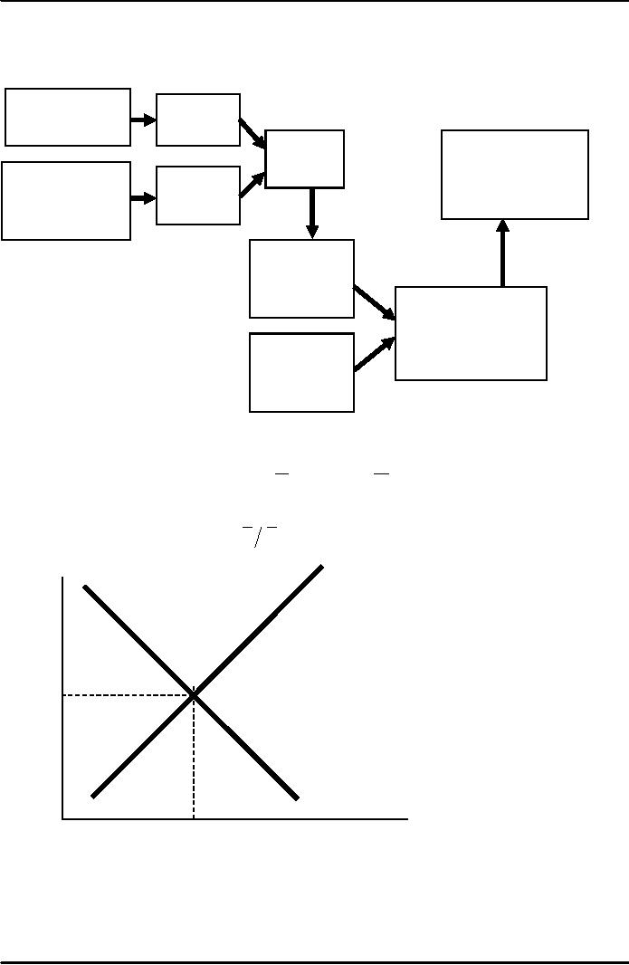
The
Big Picture
Keynesian
IS
Cross
curve
Explanation
of
IS-LM
model
short-run
Theory
of
fluctuations
LM
curve
Liquidity
Preference
Aggregate.
demand
curve
Model
of aggregate
demand
and
aggregate
supply
Aggregate.
supply
curve
Equilibrium
in the IS-LM
Model
The
IS curve represents equilibrium in
the goods market.
Y
= C
( -T
) + I
(r )
+ G
Y
The
LM curve
represents money market
equilibrium
M
P = L
(r ,Y
)
LM
r
r1
IS
Y
Y1
The
intersection determines the
unique combination of Y and r
that satisfies equilibrium in
both
markets.
122
Macroeconomics
ECO 403
VU
Policy
analysis with the IS-LM
Model
Policymakers
can affect macroeconomic
variables with
�
fiscal
policy: G
and/or
T
�
monetary
policy: M
We
can use the IS-LM
model
to analyze the effects of
these policies.
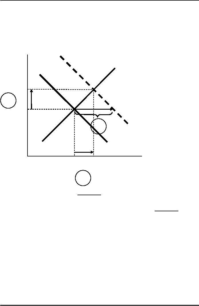
An
increase in government
purchases
r
LM
r2
2.
r1
1.
IS2
IS1
Y
Y1
Y2
3.
1
ΔG, causing
output & income to
rise.
(1-MPC)
1.
IS curve
shifts right by
1
2.
This raises money demand,
causing the interest rate to
rise
(1-MPC)
ΔG.
3.
...which reduces investment, so
the final increase in Y is
smaller than
123
Macroeconomics
ECO 403
VU
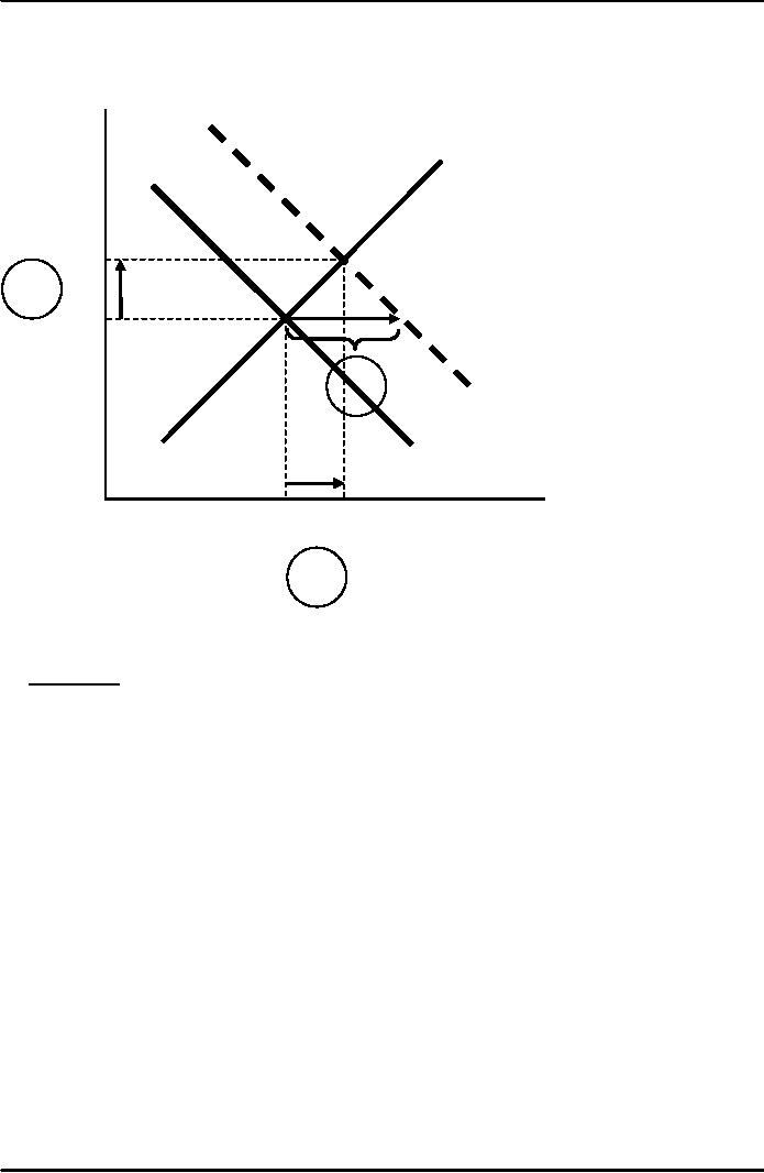
A
tax cut
r
LM
r2
2.
r1
1.
IS2
IS1
Y
Y1
Y2
2.
Because
consumers save (1-MPC) of
the tax cut, the
initial boost in spending is
smaller for ΔT
than
for an equal ΔG...
and the IS
curve
shifts by
1
ΔT
1.
(1-MPC)
2.
...so the effects on r and Y
are smaller for a ΔT than
for an equal ΔG.
124
Macroeconomics
ECO 403
VU
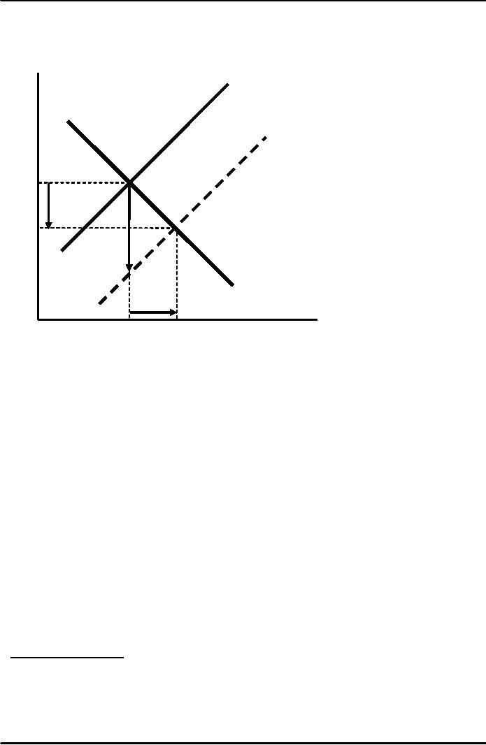
Monetary
Policy: an increase in M
r
LM1
LM2
r1
r2
IS
Y
Y2
Y1
1.
ΔM
>
0 shifts the LM
curve
down (or to the
right)
2.
...causing the interest rate
to fall
3.
...this increases investment,
causing output & income to
rise.
Interaction
between monetary & fiscal
policy
�
Model:
monetary
& fiscal policy variables
(M,
G and
T ) are exogenous
�
Real
world:
Monetary
policymakers may adjust M in
response to changes in fiscal
policy, or vice
versa.
�
Such
interaction may alter the
impact of the original
policy change.
Central
Bank's response to ΔG >
0
�
Suppose
Government increases G.
�
Possible
central bank
responses:
1.
Hold M constant
2.
Hold r constant
3. Hold
Y constant
�
In
each case, the effects of
the ΔG are
different:
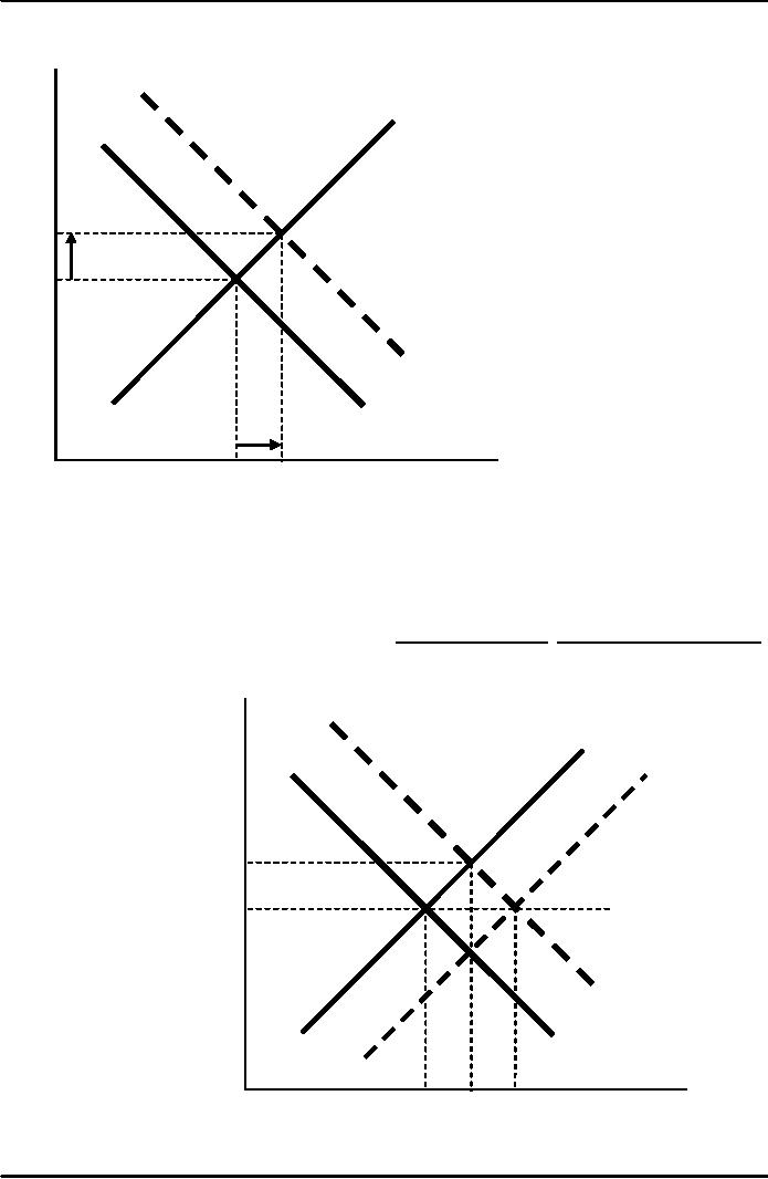
Response
1: hold M
constant
If
Government raises G,
the IS
curve
shifts right. If central
bank holds M constant, then
LM
curve
doesn't shift.
125
Macroeconomics
ECO 403
VU
r
LM1
r2
r1
IS2
IS1
Y
Y1
Y2
Results:
Δr
= r2 -
r1
ΔY
= Y
2 -
Y1
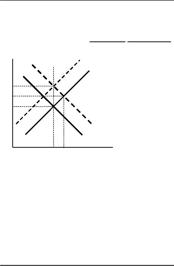
Response
2A: hold r
constant
If
Government raises G,
the IS
curve
shifts right. To keep
r
constant,
central bank increases
M
r
LM1
LM2
r2
r1
IS2
IS1
Y
Y1
Y2
Y3
to
shift LM
curve
right.
126
Macroeconomics
ECO 403
VU
ΔY
= Y
3 -
Y1
Δr
= 0
Results:
Response2B:
hold Y
constant
If
Government raises G, the
IS curve
shifts right. To keep Y
constant, central Bank
reduces M
to
shift LM
curve
left.
r
LM2
LM1
r3
r2
r1
IS2
IS1
Y
Y1
Y2
ΔY
= 0
Δr
= r3 -
r1
Results:
Shocks
in the IS-LM
Model
IS
shocks: exogenous
changes in the demand for
goods & services.
Examples:
�
Stock
market boom or crash
⇒
change in
households' wealth
⇒
ΔC
�
Change
in business or consumer
confidence
or expectations
⇒
ΔI
and/or
ΔC
127

Macroeconomics
ECO 403
VU
LM
shocks:
exogenous
changes in the demand for
money.
Examples:
�
A
wave of credit card fraud
increases demand for
money
�
More
ATMs or the Internet reduce
money demand
Analyzing
shocks with the IS-LM
model
Use
the IS-LM
model to
analyze the effects
of
A
boom in the stock market
makes consumers
wealthier.
After
a wave of credit card fraud,
consumers use cash more
frequently in transactions.
For
each shock,
Use
the IS-LM
diagram
to show the effects of the
shock on Y
and
r.
Determine
what happens to C,
I,
and the unemployment
rate.
What
is the central bank's policy
instrument?
�
What
the newspaper says:
"The
central bank lowered
interest rates by one-half
point today"
�
What
actually happened:
The
central bank conducted
expansionary monetary policy to
shift the LM curve to
the
right
until the interest rate
fell 0.5 points.
�
The
central bank targets the
discount rate: it announces a
target value, and
uses
monetary
policy to shift the LM curve
as needed to attain its
target rate.
Why
does the central bank
target interest rates
instead of the money
supply?
1)
They
are easier to measure than
the money supply
2)
The
central bank might believe
that LM shocks are more
prevalent than IS
shocks.
If
so, then targeting the
interest rate stabilizes
income better than targeting
the
money
supply.
IS-LM
and Aggregate
Demand
�
So
far, we've been using
the IS-LM
model
to analyze the short run,
when the price
level
is assumed fixed.
�
However, a
change in P would shift the
LM curve
and therefore affect
Y.
�
The
aggregate demand curve
captures this relationship
between P and Y
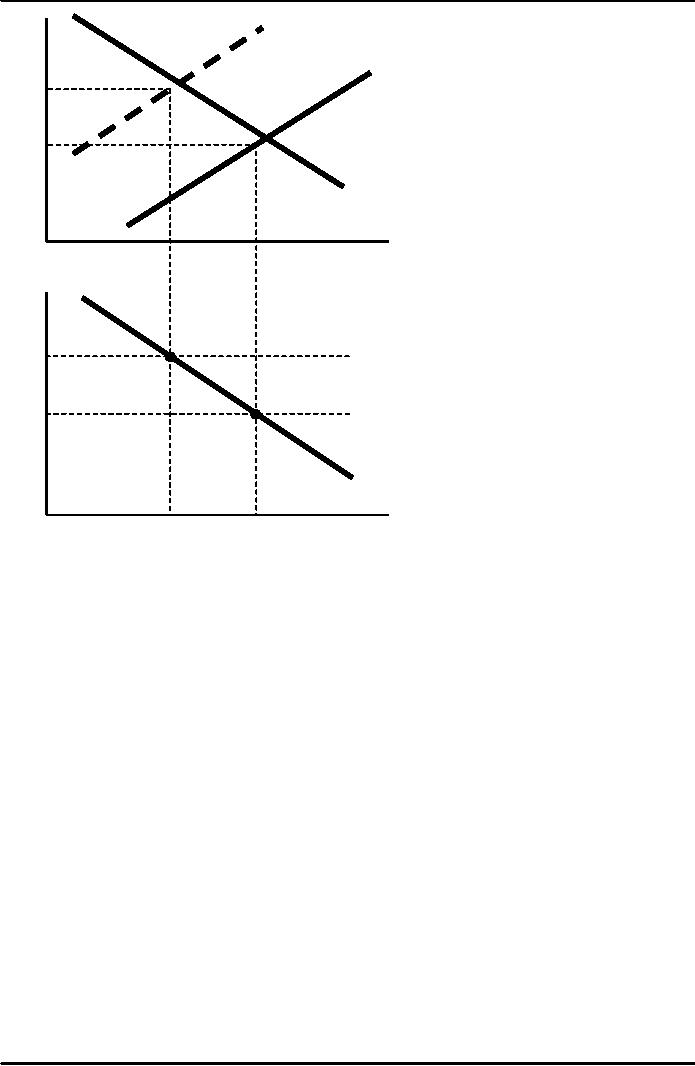
Deriving
the AD
curve
Intuition
for slope of AD
curve:
↑P
⇒
↓(M/P)
⇒
LM shifts
left
⇒
↑r
⇒
↓I
⇒
↓Y
128
Macroeconomics
ECO 403
VU
LM
(P2)
r
LM
(P1)
r2
r1
IS
Y1
Y
Y2
P
P2
P1
AD
Y
Y2
Y1
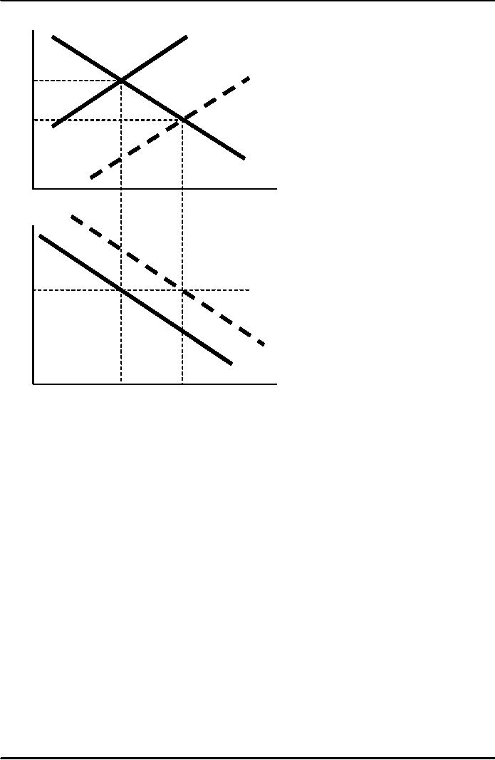
Monetary
policy and the AD
curve
The
central bank can increase
aggregate demand:
↑M ⇒
LM shifts
right
⇒
↓r
⇒
↑I
⇒
↑Y at
each value of P
129
Macroeconomics
ECO 403
VU
LM
(M1/P1)
r
LM
(M2/P1)
r1
r2
IS
Y2
Y
Y1
P
P1
AD2
AD1
Y
Y1
Y2
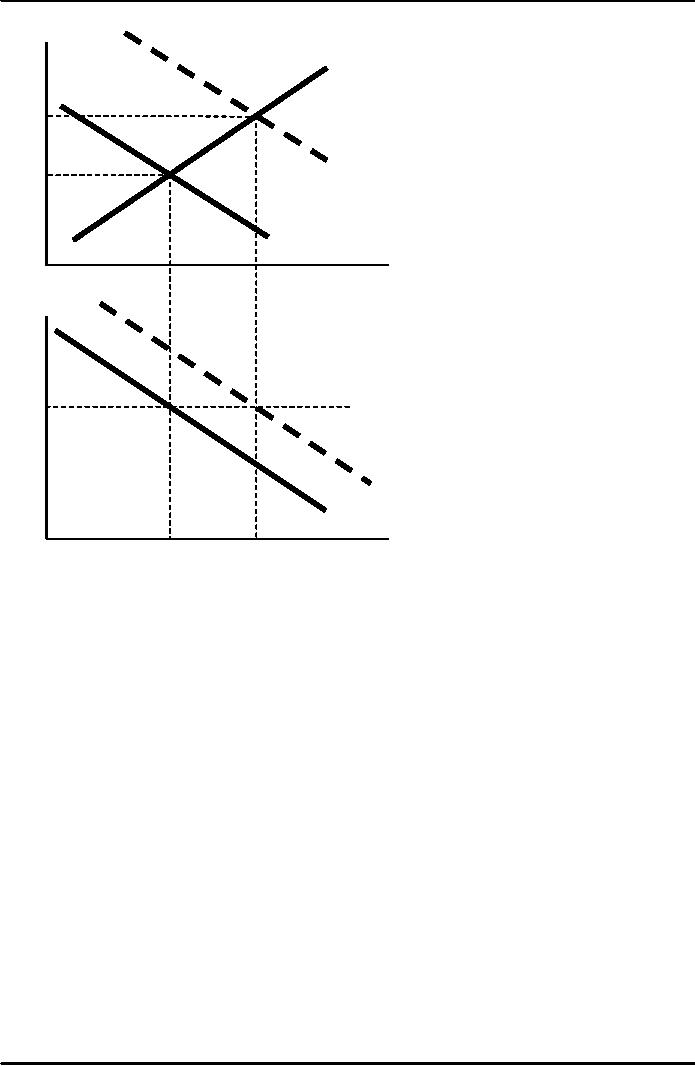
Fiscal
policy and the AD
curve
Expansionary
fiscal policy (↑G and/or
↓T)
increases
aggregate demand:
↓T ⇒
↑C
⇒
IS
shifts right
⇒
↑Y at
each value of P
130
Macroeconomics
ECO 403
VU
r
LM
r2
r1
IS2
IS1
Y
Y2
Y1
P
P1
AD2
AD1
Y
Y2
Y1
131
Table of Contents:
- INTRODUCTION:COURSE DESCRIPTION, TEN PRINCIPLES OF ECONOMICS
- PRINCIPLE OF MACROECONOMICS:People Face Tradeoffs
- IMPORTANCE OF MACROECONOMICS:Interest rates and rental payments
- THE DATA OF MACROECONOMICS:Rules for computing GDP
- THE DATA OF MACROECONOMICS (Continued…):Components of Expenditures
- THE DATA OF MACROECONOMICS (Continued…):How to construct the CPI
- NATIONAL INCOME: WHERE IT COMES FROM AND WHERE IT GOES
- NATIONAL INCOME: WHERE IT COMES FROM AND WHERE IT GOES (Continued…)
- NATIONAL INCOME: WHERE IT COMES FROM AND WHERE IT GOES (Continued…)
- NATIONAL INCOME: WHERE IT COMES FROM AND WHERE IT GOES (Continued…)
- MONEY AND INFLATION:The Quantity Equation, Inflation and interest rates
- MONEY AND INFLATION (Continued…):Money demand and the nominal interest rate
- MONEY AND INFLATION (Continued…):Costs of expected inflation:
- MONEY AND INFLATION (Continued…):The Classical Dichotomy
- OPEN ECONOMY:Three experiments, The nominal exchange rate
- OPEN ECONOMY (Continued…):The Determinants of the Nominal Exchange Rate
- OPEN ECONOMY (Continued…):A first model of the natural rate
- ISSUES IN UNEMPLOYMENT:Public Policy and Job Search
- ECONOMIC GROWTH:THE SOLOW MODEL, Saving and investment
- ECONOMIC GROWTH (Continued…):The Steady State
- ECONOMIC GROWTH (Continued…):The Golden Rule Capital Stock
- ECONOMIC GROWTH (Continued…):The Golden Rule, Policies to promote growth
- ECONOMIC GROWTH (Continued…):Possible problems with industrial policy
- AGGREGATE DEMAND AND AGGREGATE SUPPLY:When prices are sticky
- AGGREGATE DEMAND AND AGGREGATE SUPPLY (Continued…):
- AGGREGATE DEMAND AND AGGREGATE SUPPLY (Continued…):
- AGGREGATE DEMAND AND AGGREGATE SUPPLY (Continued…)
- AGGREGATE DEMAND AND AGGREGATE SUPPLY (Continued…)
- AGGREGATE DEMAND AND AGGREGATE SUPPLY (Continued…)
- AGGREGATE DEMAND IN THE OPEN ECONOMY:Lessons about fiscal policy
- AGGREGATE DEMAND IN THE OPEN ECONOMY(Continued…):Fixed exchange rates
- AGGREGATE DEMAND IN THE OPEN ECONOMY (Continued…):Why income might not rise
- AGGREGATE SUPPLY:The sticky-price model
- AGGREGATE SUPPLY (Continued…):Deriving the Phillips Curve from SRAS
- GOVERNMENT DEBT:Permanent Debt, Floating Debt, Unfunded Debts
- GOVERNMENT DEBT (Continued…):Starting with too little capital,
- CONSUMPTION:Secular Stagnation and Simon Kuznets
- CONSUMPTION (Continued…):Consumer Preferences, Constraints on Borrowings
- CONSUMPTION (Continued…):The Life-cycle Consumption Function
- INVESTMENT:The Rental Price of Capital, The Cost of Capital
- INVESTMENT (Continued…):The Determinants of Investment
- INVESTMENT (Continued…):Financing Constraints, Residential Investment
- INVESTMENT (Continued…):Inventories and the Real Interest Rate
- MONEY:Money Supply, Fractional Reserve Banking,
- MONEY (Continued…):Three Instruments of Money Supply, Money Demand