 |
AGGREGATE DEMAND AND AGGREGATE SUPPLY (Continued…): |
| << AGGREGATE DEMAND AND AGGREGATE SUPPLY (Continued…): |
| AGGREGATE DEMAND AND AGGREGATE SUPPLY (Continued…) >> |

Macroeconomics
ECO 403
VU
LESSON
26
AGGREGATE
DEMAND AND AGGREGATE SUPPLY
(Continued...)
Context
�
Model
of aggregate demand & aggregate
supply
�
Long
run
Prices
flexible
Output
determined by factors of production &
technology
Unemployment
equals its natural
rate
�
Short
run
Prices
fixed
Output
determined by aggregate
demand
Unemployment is
negatively related to
output
�
Now,
we develop the IS-LM model,
the theory that yields
the aggregate demand curve.
We
focus
on the short run and
assume the price level is
fixed.
The
Keynesian Cross
�
A
simple closed economy model
in which income is determined by
expenditure.
(due
to J.M. Keynes)
�
Notation:
I
= planned investment
E
= C + I + G
=
planned expenditure
Y
= real GDP = actual
expenditure
�
Difference
between actual & planned
expenditure: unplanned inventory
investment
Elements
of the Keynesian
Cross
C
= C
( -T
)
Y
Consumption
function:
G
= G
, T =T
Govt
policy variables:
For
now, investment is
exogenous:
I
=I
Planned
expenditure:
E
= C
( -T
) + I
+ G
Y
Actual
expenditure =
Planned
expenditure
Equilibrium
condition:
Y
= E
109
Macroeconomics
ECO 403
VU
Graphing
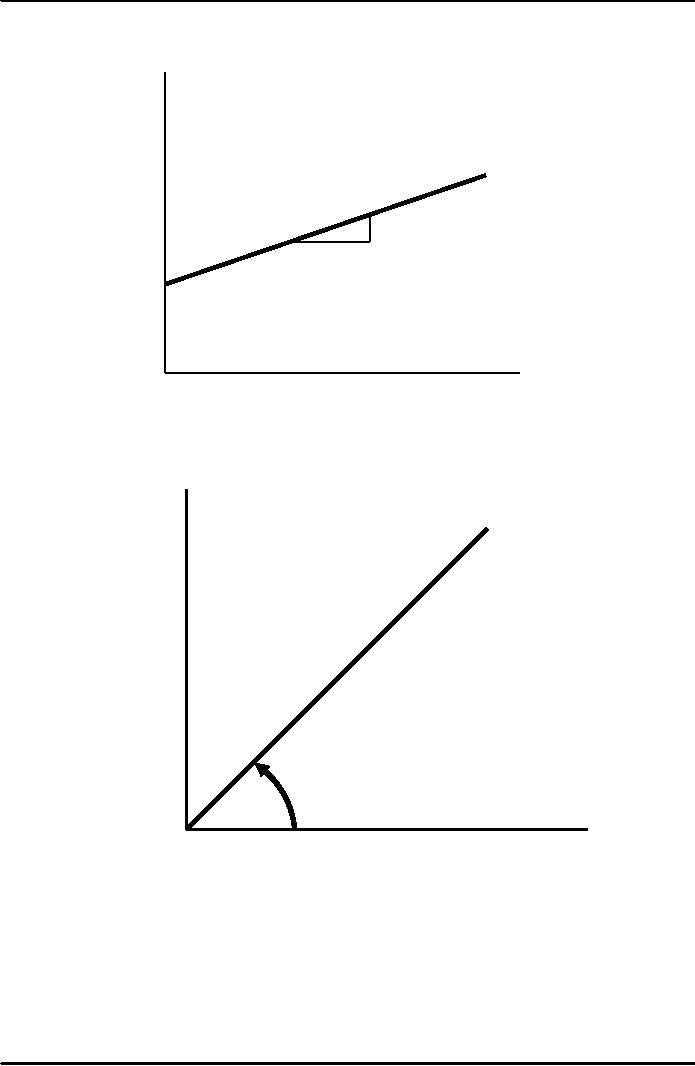
planned expenditure
E
Planned
Expenditure
E
=C +I +G
MPC
1
Income,
output, Y
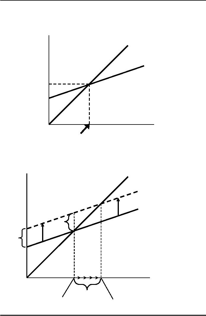
Graphing
the equilibrium
condition
E
E
=Y
Planned
expenditure
45�
Income,
output, Y
110
Macroeconomics
ECO 403
VU
The
equilibrium value of
income
E
E
=Y
Planned
Expenditure
E
=C +I +G
Income,
output, Y
Equilibrium
income
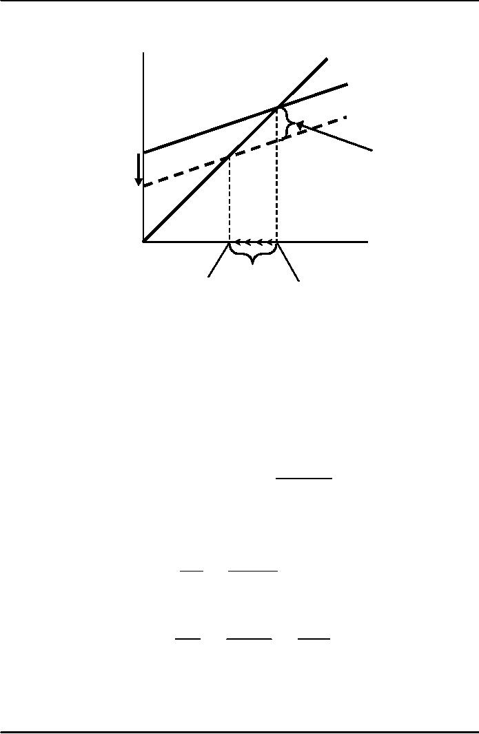
An
increase in government
purchases
E
E
=Y
E
=C +I +G2
E
=C +I +G1
ΔG
Y
ΔY
E1 = Y1
E2 = Y2
111

Macroeconomics
ECO 403
VU
At
Y1,
there is now an unplanned
drop in inventory, so firms
increase output, and income
rises
toward
a new equilibrium
Solving
for ΔY
Y
= C
+ I
+ G
Equilibrium
condition
ΔY
= ΔC
+ ΔI
+ ΔG
In
changes form
ΔC
+
ΔG
Since
I is exogenous
=
=
MPC
�
ΔY
+ ΔG
Because
ΔC =
MPC ΔY
Collect
terms with ΔY on
the left side of the
equals sign:
(1
-
MPC)
�
ΔY
= ΔG
⎛
⎞
1
Finally,
solve for ΔY:
ΔY
= ⎜
⎟
� ΔG
⎝
1
-
MPC
⎠
The
government purchases
multiplier
Example:
MPC = 0.8
1
ΔY
=
ΔG
1
-
MPC
1
1
ΔG
=
ΔG
= 5 ΔG
=
1
-
0.8
0.2
The
increase in G
causes
income to increase by 5 times as
much!
Definition:
the increase in income
resulting from a Re.1
increase in G. In this model,
the G
multiplier
equals
ΔY
1
=
ΔG
1
-
MPC
In
the example with MPC =
0.8,
ΔY
1
=
ΔG
1
-
MPC
Why
the multiplier is greater
than 1
�
ΔY
= ΔG.
Initially,
the increase in G causes an
equal increase in Y:
�
⇒
↑C
But
↑Y
⇒
Further
↑Y
⇒
Further
↑C
⇒
Further
↑Y
�
So
the final impact on income
is much bigger than the
initial ΔG.
112
Macroeconomics
ECO 403
VU
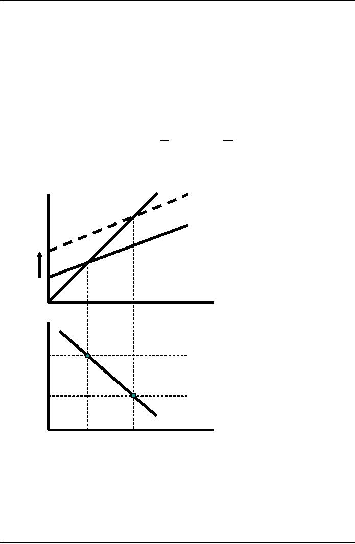
An
increase in taxes
E
E
=Y
E
=C1 +I
+G
E
=C2 +I
+G
At
Y1, there is now
an
ΔC =
-MPC
ΔT
unplanned
inventory
buildup...
Y
ΔY
E2 = Y2
E1 = Y1
Initially,
the tax increase reduces
consumption, and therefore
E:
so firms reduce output,
and
income
falls toward a new
equilibrium
Solving
for ΔY
ΔY
= ΔC
+ ΔI
+ ΔG
Equilibrium
condition in changes
I
and G are exogenous
=
ΔC
=
MPC
�
( ΔY
- ΔT
)
(1
-
MPC)
�
ΔY
= - MPC
�
ΔT
Solving
for ΔY:
⎛
- MPC
⎞
Final
result:
ΔY
= ⎜
⎟
� ΔT
⎝
1
-
MPC
⎠
The
Tax Multiplier
Definition:
the change in income
resulting from a $1 increase in
T:
ΔY
-
MPC
=
ΔT
1
-
MPC
If
MPC = 0.8, then the tax
multiplier equals
ΔY
-
0.8
-
0.8
=
=
=
-4
ΔT
1
-
0.8
0.2
Properties
of Tax Multiplier
1.
Tax multiplier is negative:
A
tax hike reduces consumer
spending, which
reduces
income.
113
Macroeconomics
ECO 403
VU
2.
Tax multiplier is greater
than one (in absolute
value): A change in
taxes has a
multiplier
effect on income.
3.
Tax multiplier is smaller
than the govt. spending
multiplier: Consumers
save the
fraction
(1-MPC) of a tax cut, so the
initial boost in spending
from a tax cut is
smaller
than
from an equal increase in
G.
The
IS curve
Definition:
a
graph of all combinations of r
and Y that result in goods
market equilibrium,
i.e.
actual
expenditure (output) = planned
expenditure
The
equation for the IS curve
is:
Y
= C
( - T
) + I
(r )
+ G
Y
Deriving
the IS
curve
E
=Y
E
E
=C +I (r2 )+G
E
=C +I (r1 )+G
ΔI
Y
Y1
Y2
r
r1
r2
IS
Y1
Y2
Y
↓r
⇒
↑I
⇒
↑E
⇒
↑Y
114
Table of Contents:
- INTRODUCTION:COURSE DESCRIPTION, TEN PRINCIPLES OF ECONOMICS
- PRINCIPLE OF MACROECONOMICS:People Face Tradeoffs
- IMPORTANCE OF MACROECONOMICS:Interest rates and rental payments
- THE DATA OF MACROECONOMICS:Rules for computing GDP
- THE DATA OF MACROECONOMICS (Continued…):Components of Expenditures
- THE DATA OF MACROECONOMICS (Continued…):How to construct the CPI
- NATIONAL INCOME: WHERE IT COMES FROM AND WHERE IT GOES
- NATIONAL INCOME: WHERE IT COMES FROM AND WHERE IT GOES (Continued…)
- NATIONAL INCOME: WHERE IT COMES FROM AND WHERE IT GOES (Continued…)
- NATIONAL INCOME: WHERE IT COMES FROM AND WHERE IT GOES (Continued…)
- MONEY AND INFLATION:The Quantity Equation, Inflation and interest rates
- MONEY AND INFLATION (Continued…):Money demand and the nominal interest rate
- MONEY AND INFLATION (Continued…):Costs of expected inflation:
- MONEY AND INFLATION (Continued…):The Classical Dichotomy
- OPEN ECONOMY:Three experiments, The nominal exchange rate
- OPEN ECONOMY (Continued…):The Determinants of the Nominal Exchange Rate
- OPEN ECONOMY (Continued…):A first model of the natural rate
- ISSUES IN UNEMPLOYMENT:Public Policy and Job Search
- ECONOMIC GROWTH:THE SOLOW MODEL, Saving and investment
- ECONOMIC GROWTH (Continued…):The Steady State
- ECONOMIC GROWTH (Continued…):The Golden Rule Capital Stock
- ECONOMIC GROWTH (Continued…):The Golden Rule, Policies to promote growth
- ECONOMIC GROWTH (Continued…):Possible problems with industrial policy
- AGGREGATE DEMAND AND AGGREGATE SUPPLY:When prices are sticky
- AGGREGATE DEMAND AND AGGREGATE SUPPLY (Continued…):
- AGGREGATE DEMAND AND AGGREGATE SUPPLY (Continued…):
- AGGREGATE DEMAND AND AGGREGATE SUPPLY (Continued…)
- AGGREGATE DEMAND AND AGGREGATE SUPPLY (Continued…)
- AGGREGATE DEMAND AND AGGREGATE SUPPLY (Continued…)
- AGGREGATE DEMAND IN THE OPEN ECONOMY:Lessons about fiscal policy
- AGGREGATE DEMAND IN THE OPEN ECONOMY(Continued…):Fixed exchange rates
- AGGREGATE DEMAND IN THE OPEN ECONOMY (Continued…):Why income might not rise
- AGGREGATE SUPPLY:The sticky-price model
- AGGREGATE SUPPLY (Continued…):Deriving the Phillips Curve from SRAS
- GOVERNMENT DEBT:Permanent Debt, Floating Debt, Unfunded Debts
- GOVERNMENT DEBT (Continued…):Starting with too little capital,
- CONSUMPTION:Secular Stagnation and Simon Kuznets
- CONSUMPTION (Continued…):Consumer Preferences, Constraints on Borrowings
- CONSUMPTION (Continued…):The Life-cycle Consumption Function
- INVESTMENT:The Rental Price of Capital, The Cost of Capital
- INVESTMENT (Continued…):The Determinants of Investment
- INVESTMENT (Continued…):Financing Constraints, Residential Investment
- INVESTMENT (Continued…):Inventories and the Real Interest Rate
- MONEY:Money Supply, Fractional Reserve Banking,
- MONEY (Continued…):Three Instruments of Money Supply, Money Demand