 |
AGGREGATE DEMAND AND AGGREGATE SUPPLY:When prices are sticky |
| << ECONOMIC GROWTH (Continued…):Possible problems with industrial policy |
| AGGREGATE DEMAND AND AGGREGATE SUPPLY (Continued…): >> |

Macroeconomics
ECO 403
VU
LESSON
24
AGGREGATE
DEMAND AND AGGREGATE
SUPPLY
Issues
under Consideration
�
Difference
between short run & long
run
�
Introduction
to aggregate demand
�
Aggregate
supply in the short run
& long run
�
See
how model of aggregate
supply and demand can be
used to analyze short-run
and
long-run
effects of "shocks"
Time
horizons
�
Long
run: Prices are flexible,
respond to changes in supply or
demand
�
Short
run: many prices are
"sticky" at some predetermined
level
The
economy behaves much
differently when prices are
sticky.
In
Classical Macroeconomic
Theory,
Recall
�
Output
is determined by the supply
side:
Supplies of
capital, labor
Technology
�
Changes
in demand for goods &
services (C, I, G ) only
affect prices, not
quantities.
�
Complete
price flexibility is a crucial
assumption, so classical theory
applies in the long
run.
When
prices are sticky
...output
and employment also depend
on demand for goods &
services, which is affected
by
�
Fiscal
policy (G
and
T)
�
Monetary
policy (M)
�
Other
factors, like exogenous
changes
in
C or
I.
�
How?
Why?
The
model of aggregate demand
and supply
�
The
paradigm that most
mainstream economists & policymakers
use to think about
economic
fluctuations and policies to
stabilize the economy
�
Shows
how the price level
and aggregate output are
determined
�
Shows
how the economy's behavior
is different in the short
run and long
run
Aggregate
demand
�
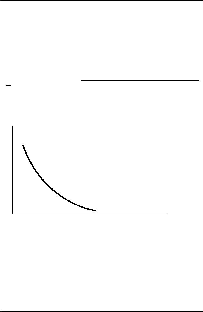
The
aggregate demand curve shows
the relationship between the
price level and
the
quantity
of output demanded.
�
For
an intro to the AD/AS model,
we use a simple theory of
aggregate demand based
on
the
Quantity Theory of
Money.
96
Macroeconomics
ECO 403
VU
�
In
the coming lectures, we
shall discuss the theory of
aggregate demand in more
detail.
The
Quantity Equation as Aggregate
Demand
�
Recall
the quantity equation
MV=PY
And
the money demand function it
implies:
(M/P)
d = k Y
where
V = 1/k
= velocity.
�
For
given values of M and V,
these equations imply an
inverse relationship between P
and
Y:
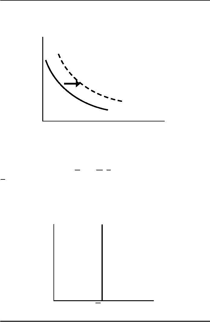
The
downward-sloping AD
curve
An
increase in the price level
causes a fall in real money
balances (M/P ), causing a
decrease
in
the demand for goods &
services.
P
AD
Y
97
Macroeconomics
ECO 403
VU
Shifting
the AD
curve
An
increase in the money supply
shifts the AD curve to the
right.
P
AD2
AD1
Y
Aggregate
Supply in the Long
Run
�
Recall
In
the long run, output is
determined by factor supplies
and technology
Y
= F
(K , L
)
Y
is the full-employment
or
natural
level
of output, the level of
output at which the
economy's
resources
are fully employed.
"Full
employment" means that
unemployment equals its
natural rate.
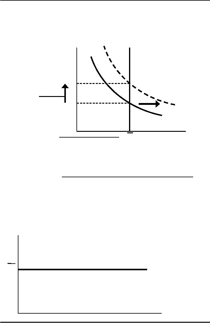
Full-employment
output does not depend on
the price level, so the
long run aggregate
supply
(LRAS) curve is
vertical:
P
LRAS
Y
Y
98
Macroeconomics
ECO 403
VU
Long-run
effects of an increase in M
An
increase in M shifts the AD
curve to the right.
P
LRAS
P2
In
the long run,
this
increases
the price
level...
P1
AD2
AD1
Y
...but
leaves output the
Y
same.
Aggregate
Supply in the Short
Run
�
In
the real world, many
prices are sticky in the
short run.
�
For
now we assume that all
prices are stuck at a
predetermined level in the
short run...
�
...and
that firms are willing to
sell as much as their
customers are willing to buy
at that price
level.
�
Therefore,
the short-run aggregate
supply (SRAS) curve is
horizontal
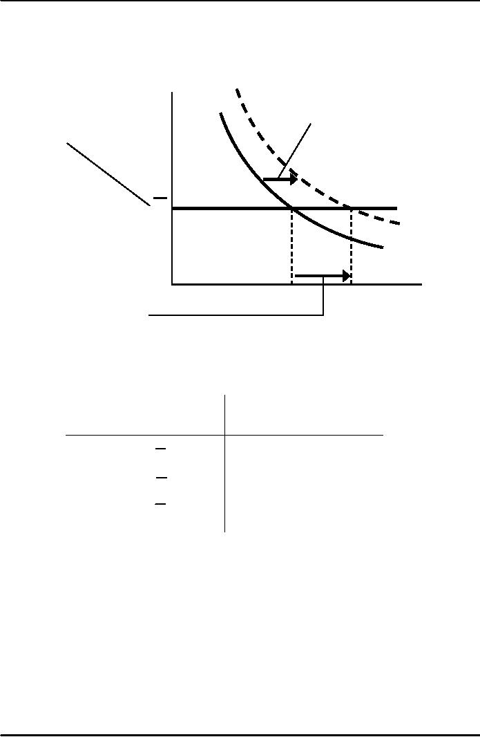
The
SRAS curve is horizontal:
The price level is fixed at
a predetermined level, and
firms sell
as
much as buyers
demand.
P
SRAS
P
Y
99
Macroeconomics
ECO 403
VU
Short-run
effects of an increase in M
P
In
the short run
when
prices
are sticky,...
...an
increase in
aggregate
demands...
SRAS
P
AD2
AD1
Y
...causes
output to rise.
Y1
Y2
From
the short run to the
long run
Over
time, prices gradually
become "unstuck." When they
do, will they rise or
fall?
In
the short-run
equilibrium,
then
over time, the
price
if
level
will
Y>Y
Rise
Y<Y
Fall
Y=Y
remain
constant
This
adjustment of prices is what
moves the economy to its
long-run equilibrium.
100
Macroeconomics
ECO 403
VU
The
SR & LR effects of ΔM >
0
P
LRAS
C
P2
B
SRAS
P
A
AD2
AD1
Y
Y2
Y
A
= initial equilibrium
B
= new short-run equilibrium
after SBP increases M
C
= long-run equilibrium
101
Table of Contents:
- INTRODUCTION:COURSE DESCRIPTION, TEN PRINCIPLES OF ECONOMICS
- PRINCIPLE OF MACROECONOMICS:People Face Tradeoffs
- IMPORTANCE OF MACROECONOMICS:Interest rates and rental payments
- THE DATA OF MACROECONOMICS:Rules for computing GDP
- THE DATA OF MACROECONOMICS (Continued…):Components of Expenditures
- THE DATA OF MACROECONOMICS (Continued…):How to construct the CPI
- NATIONAL INCOME: WHERE IT COMES FROM AND WHERE IT GOES
- NATIONAL INCOME: WHERE IT COMES FROM AND WHERE IT GOES (Continued…)
- NATIONAL INCOME: WHERE IT COMES FROM AND WHERE IT GOES (Continued…)
- NATIONAL INCOME: WHERE IT COMES FROM AND WHERE IT GOES (Continued…)
- MONEY AND INFLATION:The Quantity Equation, Inflation and interest rates
- MONEY AND INFLATION (Continued…):Money demand and the nominal interest rate
- MONEY AND INFLATION (Continued…):Costs of expected inflation:
- MONEY AND INFLATION (Continued…):The Classical Dichotomy
- OPEN ECONOMY:Three experiments, The nominal exchange rate
- OPEN ECONOMY (Continued…):The Determinants of the Nominal Exchange Rate
- OPEN ECONOMY (Continued…):A first model of the natural rate
- ISSUES IN UNEMPLOYMENT:Public Policy and Job Search
- ECONOMIC GROWTH:THE SOLOW MODEL, Saving and investment
- ECONOMIC GROWTH (Continued…):The Steady State
- ECONOMIC GROWTH (Continued…):The Golden Rule Capital Stock
- ECONOMIC GROWTH (Continued…):The Golden Rule, Policies to promote growth
- ECONOMIC GROWTH (Continued…):Possible problems with industrial policy
- AGGREGATE DEMAND AND AGGREGATE SUPPLY:When prices are sticky
- AGGREGATE DEMAND AND AGGREGATE SUPPLY (Continued…):
- AGGREGATE DEMAND AND AGGREGATE SUPPLY (Continued…):
- AGGREGATE DEMAND AND AGGREGATE SUPPLY (Continued…)
- AGGREGATE DEMAND AND AGGREGATE SUPPLY (Continued…)
- AGGREGATE DEMAND AND AGGREGATE SUPPLY (Continued…)
- AGGREGATE DEMAND IN THE OPEN ECONOMY:Lessons about fiscal policy
- AGGREGATE DEMAND IN THE OPEN ECONOMY(Continued…):Fixed exchange rates
- AGGREGATE DEMAND IN THE OPEN ECONOMY (Continued…):Why income might not rise
- AGGREGATE SUPPLY:The sticky-price model
- AGGREGATE SUPPLY (Continued…):Deriving the Phillips Curve from SRAS
- GOVERNMENT DEBT:Permanent Debt, Floating Debt, Unfunded Debts
- GOVERNMENT DEBT (Continued…):Starting with too little capital,
- CONSUMPTION:Secular Stagnation and Simon Kuznets
- CONSUMPTION (Continued…):Consumer Preferences, Constraints on Borrowings
- CONSUMPTION (Continued…):The Life-cycle Consumption Function
- INVESTMENT:The Rental Price of Capital, The Cost of Capital
- INVESTMENT (Continued…):The Determinants of Investment
- INVESTMENT (Continued…):Financing Constraints, Residential Investment
- INVESTMENT (Continued…):Inventories and the Real Interest Rate
- MONEY:Money Supply, Fractional Reserve Banking,
- MONEY (Continued…):Three Instruments of Money Supply, Money Demand