 |
Linear Programming:ARTIFICIAL VARIABLE TECHNIQUE |
| << Linear Programming:PRESENTATION IN TABULAR FORM - (SIMPLEX TABLE) |
| Linear Programming:The Two Phase Method, First Iteration >> |

Operations
Research (MTH601)
127
ARTIFICIAL
VARIABLE TECHNIQUE
If
slack variables do not
provide an initial basic
feasible solution then the
question may arise as to how
to
start
the initial table of simplex
method and proceed. This is
the case when the
slack variables have
negative values.
For
example, let us consider a
constraint
2x +
3y
> 15
The
method of converting this
inequaly (with greater than
equal to) into an equation,
is to subtract
a
slack variable
so
that we have 2x
+
3y
-
S
=
15
Now
if x
and
y
are
non-basic variables in the
problem, then S
is
taken as the starting basic
variable. But the value
of
S
=
-15 which is infeasible. We
cannot proceed with the
further iteration of the
simplex method with
infeasible basic
solution.
So
to obtain a starting solution, we
adopt the 'artificial
variable' technique. Two
methods are available
using
the
artificial variables. They
are,
(1)
The
"Big M technique" or the
Charnes method of
penalty.
(2)
The
two phase technique.
The
'Big M' Technique
If
some of the constraints in
the linear programming
problems are of the type (
>
)
or ( = ), we have to use
the
M
technique
for maximization as well as
minimization of an objective function.
The various steps of the
M
technique
are given below.
STEP
1 Express
the given linear programming
problem in the equation form
by bringing all the terms in
the
objective
function to the left hand
side and the constraints
are also expressed in the
equation form by including
slack
variables
(Add slack variable for
constraint of the type
<
and
subtract slack variable for
constraint of the type
>
).
Now
obtain a basic solution for
the problem, which will be
an infeasible one as the
basic variable is
negative
in the cases where the
constraints are of the type
( >
).
STEP
2 To
get a starting basic
feasible solution, add
n0n-negative variables to the
left hand side of each of
the
equations
corresponding to the constraints of
the types ( >
)
and ( = ). These variables
are called artificial
variables.
Thus
we change the constraint to
get a basic solution. This
violates the corresponding
constraints. This is only
for
the
starting purpose. But in the
final solution (if it
exists) if the artificial
variables will become
non-basic, (their
values
will be zero) then we are
coming back to the original
constraints. This method or
driving the
artificial
variables
out of the basis is called
the Big
M technique.
This result is achieved by assigning a
very large (big) per
unit
penalty to these variables in
the objective function. Such a
penalty will be a -M
for
maximization and a +M
for
minimization
problems, on the right hand
side, the value of M being
strictly positive. By attaching these
per unit
penalties
to the artificial variables we
ensure that they will
never become the candidates
for entering variables
once
they
are driven out.
STEP
3 For
the starting basic solution;
use the artificial variables
in the basis. Now the
starting table in the
simplex
procedure
should not contain the
terms involving the basic
variables, (one of the
conditions to be satisfied by
the
127
Operations
Research (MTH601)
128
simplex
method). But we will have
the terms like +MA
or
-MA
in
a maximization or minimization
problem
respectively
in the left hand side of
the objective row. In other
words, the objective function
must be expressed in
terms
of non-basic variables only. This
leads us to have the coefficients of
the artificial variables
(starting basic
variables)
equal to zero in objective
row. This result is obtained by
adding suitable multiples of
the constraint
equations
involving artificial variables to
the objective row.
STEP
4 Proceed
with the regular steps of
the simplex method. If the
artificial variables leave
the basis in the
final
solution,
then we come back to the
original problem. But if any
or all of the artificial
variables do not leave the
basis
in
the final solution, then
this indicates that the
problem does not have a
solution.
Example
Consider
the problem
Maximize
Z
=
2x
+
5y
Subject
to
<
40,
<
30,
x
+ y >
60,
x,
y >
0
x
y
Solution
Bring
the problem to the standard
form by including slack
variables.
STEP
1
Z
-
2x
-
5y
=0
+
S1
=
40
x
+
S2
=
30
y
x+y
+
S3 = 60
Solution
at this stage is
Z
=0
S1 =
40
⎫
⎪
S2 =
30
⎬
Basic
variables
S3 =
-60⎪
⎭
x
=
0⎫
Non-basic
variables
⎬
y
=
0⎭
STEP
2 Since
S3 = -60 and as such is
infeasible, add an artificial
variable A
to
get an initial basic
solution. Then we
x
+
y
-
S3 +
A
=
60
have
the third constraint equation
changed to
STEP
3 Modify
the objective function by including a
very large per unit penalty
M.
Thus for maximization
problem
we
add -MA
to
RHS
of
the objective function which
will be
Z
-
2x -
5
y
=
-MA
or
128
Operations
Research (MTH601)
129
Z
-
2x -
5
y
+
MA
=
0
with
the constraints
+
S1
=
40
x
+
S2
=
30
y
-
S3 + A
=
60
x+
y
Now
the required condition is that
the objective function must be
expressed in terms of the
non-basic
variables only.
Or
the coefficients of the basic
variables in the objective function
must be zero. In the
problem, the starting
basic
variables
are S1, S2 and A.
The coefficients of A
must
be made 0 in the objective function, a
result which is obtained
by
multiplying the corresponding
constraint equation including the
artificial variable by -M
and
adding to the
objective
function.
Now
Z
equation
= old Z
equation
+ (-M)
A
equation
Thus
we have the revised
objective function as,
(Z -
2x
-
5y
+
MA
=
0) + (-M)
(x
+ y -
S3 + A
=
60)
(i.e.)
Z
-
2x
-
Mx
-
5y
-
My
+
MS3 = -60 M
(i.e.)
Z
+
(-2 -
M)x +
(-5
- M)
y
+
MS3 = -60M
Now
the initial table in simplex
method is presented below
and further iterations are
carried out to obtain
a
final
feasible solution.
Starting
Table:
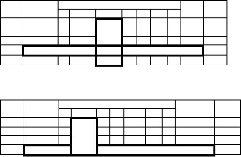
Coefficient
of
RHS
Ratio
Eqn.
Basic
No.
Variable
S1 S2
S3
A
Z
x
y
0
-
1
-2-M
-5-M
0 0
M
0
-
60M
1
0
1
0
1
0
0
0
40
∞
S1
2
0
0
1
0
1
0
0
30
30
S2
3
0
1
1
0
0
-1
1
60
60
A
First
Iteration: y enters
and S2 leaves the
basis.
RHS
Ratio
Eqn.
Basic
Coefficient
of
No.
Variable
S2
S3
A
Z
x
y
S1
0
-
1
-2-M 0
0 5+M
0
150-30M
M
1
0
1
01
0
0
0
40
40
S1
2
0
0
10
1
0
0
30
∞
y
3
0
1
00
-1
-1
1
30
30
A
129
Operations
Research (MTH601)
130
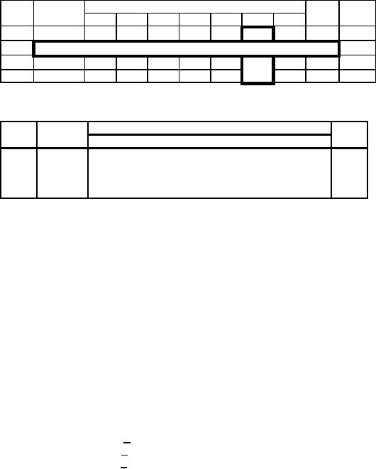
Second
Iteration: x enters
and A
leaves
the basis.
RHS
Ratio
Eqn.
Basic
Coefficient
of
No.
Variable
S2
S3
A
Z
x
y
S1
0
-
1
0
0
0
7
-2
2+M
210
1
0
0
0
1
1
1
-1
10
10
S1
2
0
0
1
0
1
0
0
30
∞
y
3
0
1
0
0
-1
-1
1
30
-30
x
Third
Iteration: S3 enters and
S1 leaves the
basis.
Eqn.
Basic
Coefficient
of
RHS
No.
Variable
S2
S3
A
Z
x
y
S1
0
-
1
0
0
2
9
0
230*
M
1
0
0
0
1
1
1
-1
10
S3
2
0
0
1
0
1
0
0
30
y
3
0
1
0
1
0
0
0
40
x
From
the above table, we see
that there is no negative coefficient in
the objective row. This
indicates that
we
have reached the optimal
solution to the problem.
Another
fact which can be noticed
that the artificial variable
A
has
left the basis.
Hence
we have the original
constraint and the original
objective function preserved.
The
optimal solution
Z*
= 230
x
=
40
y
=
30
S3 = 10
and
S1 = S2 = A
=
0
Using
surplus and artificial
variable, solve the
following:
Example
Minimize
Z
=
5x1 + 6x2
Subject
to
2x1 + 5x2 > 1500
3x1 + x2 > 1200
x1, x2 > 0
Solution
Introducing
slack (surplus) variables
S1 and S2 and artificial variables
A1 and A2 to the two constraints
the
problem
becomes,
130
Operations
Research (MTH601)
131
Minimize
Z
=
5x1 + 6x2 + MA1 + MA2
Subject
to
2x1 + 5x2 - S1 + A1 = 1500
3x1 + x2 - S2 + A2 = 1200
Since
the objective function should
not involve coefficient of basic
variables A1 and A2, we multiply the
constraint
equation with M
and
add to the objective function.
The revised objective function
will be
Z
-
5x1 + 5Mx1 - 6x2 + 6Mx2 - MS1 - MS2 = 2700M
We
prepare the simplex table as
follows:
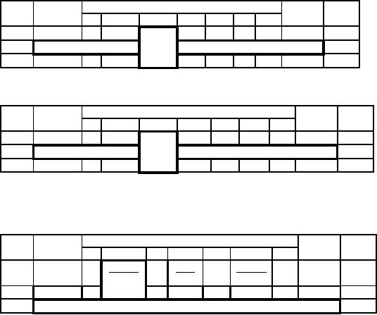
Initial
table:
RHS
Ratio
Eqn.
Basic
Coefficient
of
No.
variable
x2
S1
S2
A1
A2
Z
x1
0
-
1
5M-5
6M-6
-M -M
0
0
2700M
1
0
2
5
-1
0
1
0
1500
300
A1
2
0
3
1
0
-1
0
1
1200
1200
A2
Divide
the equation 1 by 5
throughout.
RHS
Ratio
Eqn.
Basic
Coefficient
of
No.
variable
x2
S1
S2
A1
A2
Z
x1
0
-
1
5M-5
6M-6
-M
-M
0
0
2700M
1
0
2/5
1
-1/5
0
1/5
0
300
300
A1
2
0
3
1
0
-1
0
1
1200
1200
A2
First
Iteration: x2 enters and
A1 leaves the
basis.
RHS
Ratio
Eqn.
Basic
Coefficient
of
No.
variable
x2
S1
S2
A1
A2
Z
x1
0
-
1
13M-5
0
M-1
-M
-6M+6
0
900M
5
5
5
+1800
1
0
2/5
1
-1/5
0
1/5
0
300
750
x1
2
0
13/5
-1
1/5
-1
-1/5
1
900
346
A2
Second
Iteration: x1 enters and
A2 leaves the
basis.
131

Operations
Research (MTH601)
132
Multiply
Eqn. 2 by 5/13 to make the
key number 1. Then we
have
RHS
Rati
Eqn.
Basic
Coefficient
of
o
No.
variable
x2
S1
S2
A1
A2
Z
x1
0
-
1
13M-
0
M-
-M
-
0
900M
13
1
6M+6
+1800
5
5
5
1
0
2/5
1
-
0
1/5
0
300
750
x2
1/5
2
0
1
0
1/1
-5/13
-1/13
346
346
A2
3
5/13
132
Operations
Research (MTH601)
133
Eqn.
Basic
Coefficient
of
RHS
No.
variable
x2
S1
S2
A1
A2
Z
x1
0
-
1
0
0
0
-1
-M+1
-M+1
2700M
1
0
0
1
-15/65
2/13
3/13
-2/13
2100/1
x2
3
2
0
1
0
1/13
-5/13
-1/13
5/13
4500/1
x1
3
Since
the equation 0 does not
contain positive coefficient of the
variables, the solution found is
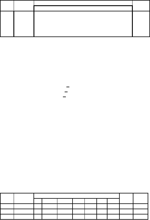
the optimum.
Z*
=
2700,
x1 = 4500 / 13,
x2 = 2100 / 13
Solution:
Example
Minimize
Z
=
4x1 + x2
Subject
to
3x1 + 4x2 > 20
-x1 - 5x2 < -15
x1, x2 > 0
Solution:
The
second constraint can be
changed into inequality of the
type by multiplying by -1 throughout.
Then
introduce
slack variable and
artificial variable to the
two constraints. The
equations are transformed
into
Z
-4x1 - x2 - MA1 - MA2
=0
3x1 + 4x2 - S1 + A1
=
20
x1 + 5x2 - S2 + A2
=
15
The
objective function should not
involve the coefficients of basic
variables A1 and A2. So, multiply
the
constraint
equation by M
and
add to the objective
equation. Then we get the
following equations.
Z
-
4x1 + 4Mx1 - x2 + 9Mx2 - MS1 - MS2
=
35M
3x1 + 4x2 - S1 + A1
=
20
x1 + 5x2 - S2 + A2
=
15
The
above equations can be
conveniently set down in the
Simplex table as shown
below.
Initial
table:
RHS
Ratio
Eqn.
Basic
Coefficient
of
No.
variable
x2
S1
S2
A1
A2
Z
x1
0
-
1
4M-4
9M-1
-M
-M
0
0
35M
1
0
3
4
-1
0
1
0
20
5
A1
2
0
1
5
0
-1
0
1
15
3
A2
133
Operations
Research (MTH601)
134
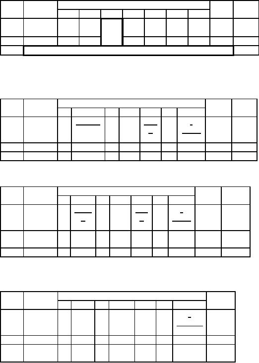
Divide
equation 2 by 5 to make the
key No. 1. Thus we
have
134
Operations
Research (MTH601)
135
RHS
Ratio
Eqn.
Basic
Coefficient
of
No.
variable
x2
S1
S2
A1
A2
Z
x1
0
-
1
4M-
9M-
-M
-M
0
0
35M
4
1
1
0
3
4
-1
0
1
0
20
5
A1
2
0
1/5
1
0
-1/5
0
1/5
3
3
A2
First
Iteration: x2 enters and
A2 leaves the
basis.
RHS
Ratio
Eqn.
Basic
Coefficient
of
No.
variable
x2 S1
S2
A1
A2
Z
x1
0
-
1
11M-19
0
-M 4M-
0
-
8M+3
5
1
9M+1
5
5
1
0
11/5
0
-1
4/5
0
-4/5
8
40/11
A1
2
2
0
1/5
1
0
-1/5
0
1/5
3
15
Multiply
the equation 1 by 5/11 to make
the key No. 1 and
the resulting table is given
below:
RHS
Ratio
Eqn.
Basic
Coefficient
of
No.
variable
x2
S1
S2
A1
A2
Z
x1
0
-
1
11M-
0
-M
-M-
0
-
8M+3
185/11
1
1
9M+1
5
5
5
1
0
1
0
-
4/11
0
-4/11
40/11
40/11
A1
5/11
2
0
1/5
1
0
-1/5
0
1/5
3
25/11
x2
Second
Iteration: x1 enters and
A1 leaves the
basis.
Ratio
Eqn.
Basic
Coefficient
of
No.
variable
x2
S1
S2
A1
A2
Z
x1
0
-
1
0
0
-
-
0
-
185/11
19/11
3/11
56M+14
25
1
0
1
0
-5/11
4/11
0
-4/11
40/11
x1
2
0
0
1
1/11
-
0
3/11
25/11
x2
3/11
Optimum
solution:
135
Table of Contents:
- Introduction:OR APPROACH TO PROBLEM SOLVING, Observation
- Introduction:Model Solution, Implementation of Results
- Introduction:USES OF OPERATIONS RESEARCH, Marketing, Personnel
- PERT / CPM:CONCEPT OF NETWORK, RULES FOR CONSTRUCTION OF NETWORK
- PERT / CPM:DUMMY ACTIVITIES, TO FIND THE CRITICAL PATH
- PERT / CPM:ALGORITHM FOR CRITICAL PATH, Free Slack
- PERT / CPM:Expected length of a critical path, Expected time and Critical path
- PERT / CPM:Expected time and Critical path
- PERT / CPM:RESOURCE SCHEDULING IN NETWORK
- PERT / CPM:Exercises
- Inventory Control:INVENTORY COSTS, INVENTORY MODELS (E.O.Q. MODELS)
- Inventory Control:Purchasing model with shortages
- Inventory Control:Manufacturing model with no shortages
- Inventory Control:Manufacturing model with shortages
- Inventory Control:ORDER QUANTITY WITH PRICE-BREAK
- Inventory Control:SOME DEFINITIONS, Computation of Safety Stock
- Linear Programming:Formulation of the Linear Programming Problem
- Linear Programming:Formulation of the Linear Programming Problem, Decision Variables
- Linear Programming:Model Constraints, Ingredients Mixing
- Linear Programming:VITAMIN CONTRIBUTION, Decision Variables
- Linear Programming:LINEAR PROGRAMMING PROBLEM
- Linear Programming:LIMITATIONS OF LINEAR PROGRAMMING
- Linear Programming:SOLUTION TO LINEAR PROGRAMMING PROBLEMS
- Linear Programming:SIMPLEX METHOD, Simplex Procedure
- Linear Programming:PRESENTATION IN TABULAR FORM - (SIMPLEX TABLE)
- Linear Programming:ARTIFICIAL VARIABLE TECHNIQUE
- Linear Programming:The Two Phase Method, First Iteration
- Linear Programming:VARIANTS OF THE SIMPLEX METHOD
- Linear Programming:Tie for the Leaving Basic Variable (Degeneracy)
- Linear Programming:Multiple or Alternative optimal Solutions
- Transportation Problems:TRANSPORTATION MODEL, Distribution centers
- Transportation Problems:FINDING AN INITIAL BASIC FEASIBLE SOLUTION
- Transportation Problems:MOVING TOWARDS OPTIMALITY
- Transportation Problems:DEGENERACY, Destination
- Transportation Problems:REVIEW QUESTIONS
- Assignment Problems:MATHEMATICAL FORMULATION OF THE PROBLEM
- Assignment Problems:SOLUTION OF AN ASSIGNMENT PROBLEM
- Queuing Theory:DEFINITION OF TERMS IN QUEUEING MODEL
- Queuing Theory:SINGLE-CHANNEL INFINITE-POPULATION MODEL
- Replacement Models:REPLACEMENT OF ITEMS WITH GRADUAL DETERIORATION
- Replacement Models:ITEMS DETERIORATING WITH TIME VALUE OF MONEY
- Dynamic Programming:FEATURES CHARECTERIZING DYNAMIC PROGRAMMING PROBLEMS
- Dynamic Programming:Analysis of the Result, One Stage Problem
- Miscellaneous:SEQUENCING, PROCESSING n JOBS THROUGH TWO MACHINES
- Miscellaneous:METHODS OF INTEGER PROGRAMMING SOLUTION