Inventory Control:SOME DEFINITIONS, Computation of Safety Stock

<< Inventory Control:ORDER QUANTITY WITH PRICE-BREAK

Linear Programming:Formulation of the Linear Programming Problem >>

Operations Research (MTH601)

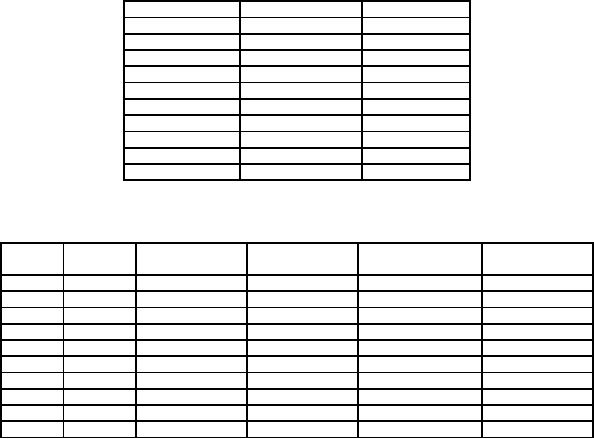
STEP 1: Calculate usage value by multiplying annual usage of each item with its unit cost and tabulate them and

assign rank by giving rank to the largest usage value as in table below.

Items No.

Annual Usage

Ranking

3000

40500

300

5000

200

22000

800

4000

9000

700

STEP 2: Arrange items as per ranking and calculate cumulative usage and % cumulative value as in the table below.

% of cumulative

Cumulative %

Rank

Item No.

Annual usage

Cumulative

Annual usage

of item

40500

22000

62500

9000

71500

5000

76500

4000

80500

94.2

3000

83500

800

84300

98.6

700

85000

99.4

300

85300

99.8

200

85500

100

If you draw the figure, you will see that the curve changes at points (say) X and Y. The items upto X is classified as

class A items and between X and Y as class B and the rest as class C items.

SOME DEFINITIONS

Lead-time: This is defined as the time interval between the placing of the orders and the actual receipt of goods.

Lead-time Demand: This is the lead-time multiplied by demand rate. For example, if the lead-time is 3 weeks and

the demand is at the rate of 50 items per week, then the lead-time demand is 3 x 50 = 150 items.

The lead-time may not be constant. For one batch, a vendor may take 45 days and for the next batch 50 days and so

on. Lead-time itself is therefore a stochastic variable. This complicates the problem of accumulating stock over the

period encompassed by the lead-time. Lead-time may also be forecast exponentially as is done with the demand.

Safety stock or Buffer stock: Lead-time demand is the stock level, which, on the average is sufficient to satisfy the

customer's orders as the stocks are being replenished. "On the average" would mean that during this period of

replenishment 50% of the customer's order can be filled and the remaining 50% may either be refused or back

ordered to be filled later. The reason for this is obvious. Forecast is after all a point estimate only. If the demand is

Operations Research (MTH601)

greater than the forecasts, the customers would not be serviced. If the demand is less then the forecasts,

overstocking would occur. When these two variables, stock level and service to the customer, are summed up over

thousands of stock level and service to the customer, are becomes a major problem for an organisation to find an

acceptable compromise between the two. Sometimes the management in an organisation would like to limit the

disservice to the customer down to 5% or 10% at the cost of extra stocking. This extra stock in excess of the lead-

time demand is called the safety stock. Saftely stock may be expressed as percentages of the lead-time demand. It

may be computed in different ways.

Reorder level: This is defined as the level of the inventory at which the order is placed. It has generally two

components (i) Lead time Demand and (ii) Safety Stock.

Reorder level (ROL) = Lead time demand (LTD) + Safety stock (SS).

Computation of Safety Stock:

As discussed earlier, if the demand exceeds the forecast, the result is bad service to the customer and if the demand

is less than the forecast figure, this results in overstocking. Thus there is a forecast error. This error is assumed to be

normally distributed, with zero mean. If the standard deviation of the forecast error is calculated, then safety stock

may be set with the desired confidence level to result in not more the 5 or 10% shortages etc.

There is another measure of variation, popularly known as mean absolute deviation (MAD), which can be computed

far more easily. It can be routinely smoothed every period for obtaining better estimates of the safety stock.

MAD is related to the standard deviation for a normal distribution as given by.

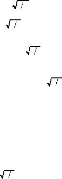
MAD = 2 š SD.

SD = š 2MAD

Therefore,

Now safety stock = Z (S.D)

= Z š 2MAD

= K MAD

where K is called service factor K = Z š 2

The safety stock is for just one period and has to be extended over the lead time. The necessary formula has been

derived by extensive simulation by statisticians and is given below.

MADLT = (0.659+ 0.341 LT) MAD

Safety stock over the lead-time

= K (0.659 + 0.341 LT ) MAD

= Z š 2 (0.659 + 0.34 LT )MAD

Example: A company uses annually 50000 units of raw materials at a cost Rs. 1.2 per item. Ordering cost of items is

Rs. 45 per order and item carrying cost is 15% per year of the average inventory.

Operations Research (MTH601)

Find the economic quantity.

Suppose that the company follows the EOQ policy and it operates for 300 days a year, that the

procurement time is 12 days and mum, minimum and average inventories.

Solution:

D = Demand = 50000/year

No. of days = 300/year

C1 = Rs. 1.2 per item

Lead time = 12 days

C2 = Rs. 45 per order

Safety stock = 500

C3 = 15% of Rs. 1.2/item/year.

= Rs. 0.18 per item per year.

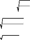
2C2D

EOQ =

(1)

2×45×50000

0.18

= 25000000

= 5000

(2)

Requirement per day = 50000/300

Lead time demand = 12 x 500/3 = 2000

Safety stock

= 500

Reorder level

= Lead time demand + safety stock

= 2000 + 500 = 2500

Maximum inventory = E.O.Q + Safety stock

= 5000 + 500 = 5500

Minimum inventory = Safety stock = 500

Average inventory

= (Max. Inv. + Min. Inv.)/2

= (5500 + 500)/2 = 3000

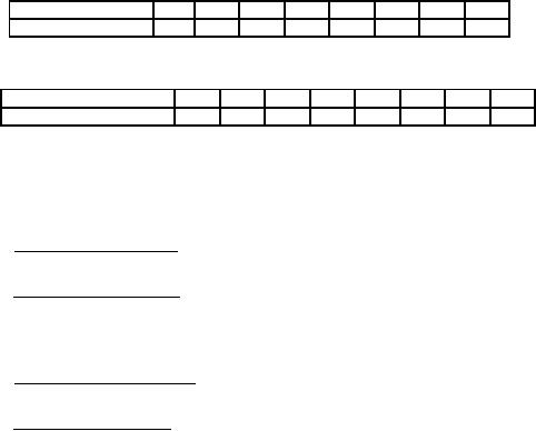
Example A scrutiny of past records gives the following distributions for lead time and daily demand during lead time.

Lead time distribution

Operations Research (MTH601)

Lead time (days)

Frequency

Demand distribution

Demand/day (units)

Frequency

What should be the buffer stock?

Solution:

Computation of average or mean lead time.

∑ (Frequency × lead time)

∑ Frequency

6+12+20+24+14+6+18+10

= 6 days

Average demand

∑ (Frequency × demand/day)

∑ frequency

0+4+10+15+16+10+6+14

Average lead-time demand

= Average lead time x Average demand/day

= 6 x 3 = 18.

Maximum lead-time demand.

= Max. lead time x Max. demand/day

= 10 x 7 = 70

∴ Buffer stock = Max. lead time demand - Average lead time demand

*Example 7.7.3

For a fixed order quantity system find the EOQ, SS, ROL and average inventory for an item with the

following data.

Demand = 10000 units

Cost of item = Re. 1

Order cost = Rs. 12

Operations Research (MTH601)

Holding cost = 24%

Post lead times = 13 days

Solution:

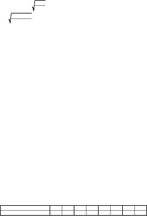
2C2D

EOQ =

(1)

2×12×10000

= 1000 items

0.24×1

(2)

The Average lead time = (13 + 14 + 15 + 16 + 17)/5

= 15 days ( 30 days time is omitted)

Maximum lead time = 30 days

Safety stock = ( 30 - 15) x 10000/(30 x 12) = 420

(3)

Reorder level = Lead time demand + Safety stock

= 417 + 420 = 837

(4)

Average inventory = (1420 + 420)/2

= 1840/2 = 920.

Example: An airline has determined that 10 spare brake cylinders will give them stock out risk of 30%, whereas 14

will reduce the risk to 15% and 16 to 10%. It takes 3 months to receive items from supplier and the airline has an

average of 4 cylinders per month. At what stock level should they reorder assuming that they wish to maintain an

85% service level.

Solution:

Lead time demand = 3 x 4 = 12 items

Safety stock at 85% service

= 15% disservice

or 15% stock out risk

= 14 items

Reorder level = 12 + 14 = 26 items.

Example: Data on the distribution of lead time for a motor component were collected as shown. Management would

like to set safety stock levels that will limit the stock out to 10%.

Lead time (weeks)

Frequency of occurrence

Operations Research (MTH601)

How many weeks of safety stock are required to provide the desired service level?

Solution:

Lead time (weeks)

Frequency

Probability

Cumulative

Probability

0.05

0.10

0.15

0.35

0.50

0.20

0.70

0.15

0.85

0.05

0.90

0.05

0.95

0.05

1.00

200

Average lead time = ∑ (lead time x frequency)/ ∑ frequency

= (10 + 40 + 210 + 160 + 150 + 60 + 70 + 80)/200

= 770/200 = 3.85 weeks

Upto 90% service level max. lead time is 6 weeks.

Hence 6 - 3.85 = 2.15 weeks of stock would provide the service level of 90%

(Note: If the lead time is given as a continuous time distribution take the mid point.)

Example: Demand for a product during an order period is assumed to be normally distributed with mean of 1000

units and standard deviation of 40 units. What % service can a company expect to provide (i) if it satisfies the

average demand only (ii) if it carries a safety stock of 60 units.

Solution:

If the company provides only average demand, we can expect only 50% service level.

The standard normal variate Z is computed with the following formula.

Z = (Safety stock - 0)/ Standard deviation

= (60 - 0)/40 = 1.5

The area under normal curve for Z = 1.5 is 0.4332.

∴ Service level = 0.50 + 0.4332 = 0.9332

04 93.32%

Example: A manufacturer of water filters purchases components in EOQ's of 850 units/order. Total demand

averages 12000 components per year and MAD = 32 units per month. If the manufacturer carries a safety stock of 80

units, what service level does the this give the firm?

Solution:

Operations Research (MTH601)

2 × MAD = MAD / 0.8 = 32 / 0.8 = 40

Standard deviation =

Z = (S S - 0)/S.D = (80 - 0)/40 = 2

The area under normal curve for Z = 2 = 0.4772.

Service level = 0.9772 or 97.72%

Example: A firm has normally distributed forecast of usage with MAD = 60 units. It desires a service level, which

limits the stock, outs to one order cycle per year.

(1) How much safety stock should be carried if the order quantity is normally a week's supply?

(2) How much safety stock should be carried if the order quantity is weeks supply.

Solution:

No. of orders = 52/year.

1 stock out in 52 weeks means a 98 % = (51/52) values

For 98% area, the value of

Z = 2.05 (from tables)

S D = MAD/0.8 = 60/08

Z = (S S - 0 )/S D= (S S - 0)/60/0.8

2.05 = (S S - 0 ) x 0.8/60

SS = 2.05 x 60/0.8 = 154 units.

(a) Number of orders = 52/5

1 stock out = (52/5 - 1)

Service level = (47/5)/(52/5) = 47/52 = 0.904

Z = 1.285 (for area = 0.404) MAD = 60

1.285 = S S/75

S S = 75 x 1.285 = 96 units.

Table of Contents: