Inventory Control:ORDER QUANTITY WITH PRICE-BREAK

<< Inventory Control:Manufacturing model with shortages

Inventory Control:SOME DEFINITIONS, Computation of Safety Stock >>

Operations Research (MTH601)

ORDER QUANTITY WITH PRICE-BREAK

The concept of Economic Order Quantity fails in certain cases where there is a discount offered when purchases are

made in large quantities. Certain manufacturers offer reduced rate for items when a larger quantity is ordered. It may

appear that the inventory holding cost may increase if large quantities of items are ordered. But if the discount offered

is so attractive that it even outweighs the holding cost, the probably the order at levels other than the EOQ would be

economical. An illustration is given in the following example and the rationale is explained.

Example: A company uses 12000 items per year supplied ordinarily at a price of Rs. 3.00 per item. Carrying costs

are 16% of the value of the average inventory and the ordering costs are Rs. 20 per order. The supplier however

offers discounts as per the table below:

Order size

Price per item

Less than 2000

Rs. 3.00

2000 to 3999

Rs. 290

4000 or more

Rs. 2.85

Compute the economic order size.

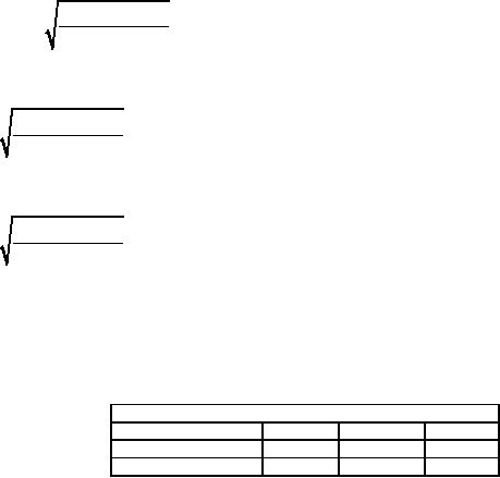
2 ×12000 × 20

EOQ =

= 1000

3.00 × 0.16

EOQ at Rs. 2.90 per item

2 ×12000 × 20

= 1017

2.90 × 0.16

EOQ at Rs. 2.85 per item

2 ×12000 × 20

= 1026

2.85 × 0.16

The EOQ at Rs. 2.90 per item = 1017. But the price per item is Rs. 2.9 only if the items are ordered in the range of

2000 to 3999. This is therefore an infeasible solution. Similarly the EOQ at Rs. 2.85 per item is 1026. This price is

valid only for items ordered in the range 4000 or more. This is also an infeasible solution.

We follow the routine procedure and calculate the cost for various order sizes: 1000, 2000, 4000,

Order size

1000

2000

4000

Item cost (Rs.)

36000

34800

34200

Order cost (Rs.)

240

120

Holding cost (Rs.)

240

464

912

Operations Research (MTH601)

Exercises

1. Assume the following price structure

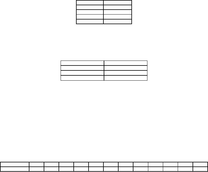
Units

Units Price

0-199

Rs. 10.00

200-399

9.75

400-599

9.50

600

9.25

Purchase cost per order

= Rs. 25

Cost of the item

= Rs. 10

Annual demand

= 950 Units

Carrying cost

= Rs. 2/Unit/year

2. Find the optimal order quantity for a product for which the price-breaks are as follows:

Items

Price/Unit

0≤

Rs. 20

q < 100

100 ≤

Rs. 18

q < 200

200 ≤

Rs. 16

The monthly demand for the product is 600 units. The storage cost is 15% of unit cost and the cost

of ordering is Rs. 30 per order.

DYNAMIC ORDER QUANTITY

The basic assumption in the derivation of Economic Order Quantity models discussed previously is that the

demand is uniform. But in certain situations the demand is not uniform. It may rise and fall, depending on seasonal

influences. A general method is discussed below that can be applied to any pattern of varying demand due to

seasonal or irregular variations.

Consider the following example to illustrate how a varying demand problem can be tackled. This is known as

Dynamic Order Quantity model.

Example: The requirements for 12 months are given below:

Month

Requirement

Set up cost

= Rs. 20

Unit price

= Rs. 5 per item.

Interest

= 24% per year

or 2% per month.

Solution: To calculate the dynamic order quantity we can adopt the following procedure.

Operations Research (MTH601)

The first month's requirement has to be ordered in the first month itself at a procurement cost of Rs. 20. Now we

have to decide whether the second month's requirement can also be ordered along with first month's requirement.

This involves additional carrying cost, but this will result in saving an extra set up. Hence if the saving on set up costs

outweighs the carrying costs, then we include the second month's requirements along with the first month. Similarly a

decision can be taken whether to include the third month's requirement in the first month itself. This procedure is

followed until the procurement costs and carrying costs are balanced.

Let n represent the month, n = 1, 2, ..., 12. Let Rn be the requirement during nth month and Rn+1 be the

requirement during (n + 1)th month. If the (n + 1)th month requirement namely Rn+1 is absorbed in nth month itself,

the additional procurement cost is saved.

Hence the saving in procurement cost is (C2/n). But the additional carrying cost is C3 n (Rn+1). If the

additional carrying cost is less than the procurement cost, then the (n+1)th month requirement is to be ordered also

with nth month.

Hence we have to check whether

n Rn + 1 C3 < C2/n

n2 Rn + 1 < C2/C3

If the answer to the above inequality is yes, then, the future month's requirements are included in the first month itself.

If the answer is 'no', then that requirement is to be ordered afresh and this is treated as month

n = 1. In this

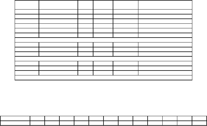
example C2/C3 = 20/0.01 = 200. All the eleven information can be represented in the table as shown.

n2Rn+1.

Month.

Requirement. Rn

n Rn+1<200

Action.

Yes

include 40 in month 1

Yes

include 10 in month 1

Yes

include 10 in month 1

160

Yes

include 10 in month 1

Yes

include 2 in month 1

1440

set up again in month 7

Total

Yes

include 10 in 7th month.

160

Yes

include 40 in 7th month.

360

set up again in month 10

Total

110

Yes

include 10 in month 10

Yes

include 20 in month 10

Total

Hence we order three times a year in the first month, seventh month and tenth month, the batch sizes being 92, 110

and 70 respectively.

Exercise: Compute the dyanamic EOQ is for the following requirements.

Month

Requirement.

100

170

150

180

260

100

150

200

Operations Research (MTH601)

ABC ANALYSIS

The ABC analysis is the analysis that attracts management on those items where the greatest savings can be

expected. This is a simple but powerful tool of statistical sampling in the area of inventory control or materials

management.

In this analysis, the items are classified or categorized into three classes, A, B and C by their usage value. The usage

value is defined as,

The ABC concept is based on Pareto's law that few high usage value items constitute a major part of th capital

invested in inventories whereas a large number of items having low usage value constitute an insignificant part of the

capital. It too much inventory is kept, the ABC analysis can be performed on a sample. After obtaining the random

sample the following steps are carried out for the ABC analysis.

STEP 1: Compute the annual usage value for every item in the sample by multiplying the annual requirements by

the cost per unit.

STEP 2: Arrange the items in decending order of the usage value calculated above.

STEP 3: Make a cumulative total of the number of items and the usage value.

STEP 4: Convert the cumulative total of number of items and usage values into a percentage of their grand totals.

STEP 5: Draw a graph connecting cumulative % items and cumulative % usage value. The graph is divided

approximately into three segments, where the curve sharply changes its shape. This indicates the three segments A,

B and C.

The class A items whose usage values are higher are to be carefully watched and are under the strict and continued

scrutiny of the senior inventory control staff. These items should be issued only an indents sanctioned by the staff.

The class C items on the other extreme can be placed on the shop floor and the personnel can help themselves

without placing a formal requisition. The class B items fall in between A and C.

ABC concept conforms to the consideration implied in the EOQ model. 'A' items have high inventory carrying

costs and should therefore be placed with EOQ concept. The 'C' items require very little capital and have therefore

low inventory carrying costs. Hence, they can be purchased in bigger lots. 'B' items are usually placed under

statistical stock control.

Example: Perform ABC analysis on the following sample of 10 items from an inventory.

Items

Annual

Usage

300

2700

1000

220

160

800

600

(Unit)

Unit

Cost

100

(Rs.)

Solution:

Table of Contents: