 |
Inventory Control:Manufacturing model with no shortages |
| << Inventory Control:Purchasing model with shortages |
| Inventory Control:Manufacturing model with shortages >> |

Operations
Research (MTH601)
63
Rs.5�747�0.5
=
Shortage
cost
2�12
=
Rs.
77.75 per order
Total
cost per order
=
3857
+
400
+
77.75
+
322.14
=
Rs.
4656.89
Annual
cost =
Number
of orders/year �
cost
=
4.66
�
4656.89
=
Rs.
21701.
Model
3: Manufacturing model with no
shortages
In
this model the following
assumptions are made:
(1)
Demand
is at a constant rate (D).
All
cost coefficients (C1, C2,
C3)
are constants.
(2)
(3)
There
is no shortage cost, or C4 = 0.
(4)
The
replacement rate is finite
and greater than the
demand rate. This is also
called replenishment
rate
or
manufacturing rate, denoted by
R.
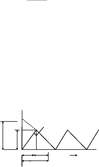
Schematically,
this model is illustrated in
fig 4
Slope=
(R-D)
Slope
= D
Q
Im
t2
Time
t1
t
Fig.
4
The
total cost of inventory per
period is the sum of three
components: item cost, order
cost and items holding
cost.
Let
Im be the
maximum inventory, t1 be
the time of manufacture and
t2 be
the time during which
there is no supply.
In
this model, all items
required for a cycle are
not stored at the beginning
as in Wilson's Model. The
items are
manufactured
at a higher rate than the
demand so that the
difference (RD)
is the existing inventory
till the items
are
exhausted.
Item
cost/period = C1Q
(32)
Order
cost/period = C2
(33)
63

Operations
Research (MTH601)
64
=
C
�
I
� (t1 +
t2 ) 2
Item
holding cost/period
(34)
m
3
=
C3 I
m � t
2
(35)
=
t
(
R
-
D)
(36)
I
1
m
t
=Q
R
(37)
But
1
=
(Q
R)(
R
-
D)
Therefore
(38)
I
m
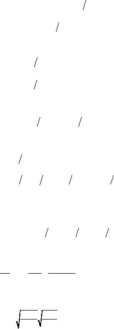
Substituting
the value of Im, we get
the total cost of inventory
per period.
C′
= C
Q +
C2 +
C3 (Q
R)( R
-
D) �
t
2
(39)
1
Total
cost of inventory per unit
time
C
=
C′
t
(40)
t
+
C3 (Q
R)( R
-
D) �
t
=
C
Q t +C
(41)
2
1
2
But
t =
Q/D
Substituting
the value of t
we
get
C
=
C
D +
C
D Q +
C3 (Q
R) ( R-D)
2
(42)
1
2
Differentiating
C
with
respect to Q
and
setting equal to zero for
minimum C,
we get,
C
D C (
R-D)
dC
=
0-
2
+
3
=0
(43)
dQ
2R
Q2
Solving
equation (43), we get
2C2D
R
Q*
=
(44)
R-D
C3
This
gives the economic order
quantity and is a balance
between holding and set up
costs.
64

Operations
Research (MTH601)
65
Example:
The demand for an item in a
company is 18000 units/year
and the company can
produce at the rate
of
3000
per month. The cost of
one set up is Rs. 500
and the holding cost of 1
unit per month is 15 paisas.
Determine:
(a)
The
optimum manufacturing
quantity.
(b)
The
maximum inventory.
(c)
The
time between orders.
(d)
The
number of orders/year.
(e)
The
time of manufacture.
(f)
The
optimum annual cost if the
cost of the item per
unit is Rs. 2.
Assume
no shortages.
Solution
C1 = Rs. 2
per item.
C2 = Rs. 500
per order.
C3 = Rs. 0.15
per item per
month
D
= 18000/year =
1500/month
R
=
3000/month
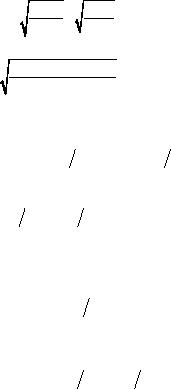
a)
Optimum
manufacture quantity
2C2D
R
Q*
=
R-D
C3
2�500�1500�3000
=
=
4470
units
C
0.15(3000-1500)
b)
The
maximum inventory
=
Q
(
R-D)
R
=
4470
�
1500
3000 =
2235
units
I
m
c)
The
time between orders
t
=
Q
D =
4470
1500 =
2.98
months
3
months
d)
The
number of orders/year
N
=
12
3 =
4
e)
The
time of manufacture
t
=
Q
R =
4470
3000 =
1.490
months
1
f)
The
optimum annual cost
=
Item cost + Ordering cost +
Holding cost
65
Table of Contents:
- Introduction:OR APPROACH TO PROBLEM SOLVING, Observation
- Introduction:Model Solution, Implementation of Results
- Introduction:USES OF OPERATIONS RESEARCH, Marketing, Personnel
- PERT / CPM:CONCEPT OF NETWORK, RULES FOR CONSTRUCTION OF NETWORK
- PERT / CPM:DUMMY ACTIVITIES, TO FIND THE CRITICAL PATH
- PERT / CPM:ALGORITHM FOR CRITICAL PATH, Free Slack
- PERT / CPM:Expected length of a critical path, Expected time and Critical path
- PERT / CPM:Expected time and Critical path
- PERT / CPM:RESOURCE SCHEDULING IN NETWORK
- PERT / CPM:Exercises
- Inventory Control:INVENTORY COSTS, INVENTORY MODELS (E.O.Q. MODELS)
- Inventory Control:Purchasing model with shortages
- Inventory Control:Manufacturing model with no shortages
- Inventory Control:Manufacturing model with shortages
- Inventory Control:ORDER QUANTITY WITH PRICE-BREAK
- Inventory Control:SOME DEFINITIONS, Computation of Safety Stock
- Linear Programming:Formulation of the Linear Programming Problem
- Linear Programming:Formulation of the Linear Programming Problem, Decision Variables
- Linear Programming:Model Constraints, Ingredients Mixing
- Linear Programming:VITAMIN CONTRIBUTION, Decision Variables
- Linear Programming:LINEAR PROGRAMMING PROBLEM
- Linear Programming:LIMITATIONS OF LINEAR PROGRAMMING
- Linear Programming:SOLUTION TO LINEAR PROGRAMMING PROBLEMS
- Linear Programming:SIMPLEX METHOD, Simplex Procedure
- Linear Programming:PRESENTATION IN TABULAR FORM - (SIMPLEX TABLE)
- Linear Programming:ARTIFICIAL VARIABLE TECHNIQUE
- Linear Programming:The Two Phase Method, First Iteration
- Linear Programming:VARIANTS OF THE SIMPLEX METHOD
- Linear Programming:Tie for the Leaving Basic Variable (Degeneracy)
- Linear Programming:Multiple or Alternative optimal Solutions
- Transportation Problems:TRANSPORTATION MODEL, Distribution centers
- Transportation Problems:FINDING AN INITIAL BASIC FEASIBLE SOLUTION
- Transportation Problems:MOVING TOWARDS OPTIMALITY
- Transportation Problems:DEGENERACY, Destination
- Transportation Problems:REVIEW QUESTIONS
- Assignment Problems:MATHEMATICAL FORMULATION OF THE PROBLEM
- Assignment Problems:SOLUTION OF AN ASSIGNMENT PROBLEM
- Queuing Theory:DEFINITION OF TERMS IN QUEUEING MODEL
- Queuing Theory:SINGLE-CHANNEL INFINITE-POPULATION MODEL
- Replacement Models:REPLACEMENT OF ITEMS WITH GRADUAL DETERIORATION
- Replacement Models:ITEMS DETERIORATING WITH TIME VALUE OF MONEY
- Dynamic Programming:FEATURES CHARECTERIZING DYNAMIC PROGRAMMING PROBLEMS
- Dynamic Programming:Analysis of the Result, One Stage Problem
- Miscellaneous:SEQUENCING, PROCESSING n JOBS THROUGH TWO MACHINES
- Miscellaneous:METHODS OF INTEGER PROGRAMMING SOLUTION