 |
Inventory Control:Purchasing model with shortages |
| << Inventory Control:INVENTORY COSTS, INVENTORY MODELS (E.O.Q. MODELS) |
| Inventory Control:Manufacturing model with no shortages >> |

Operations
Research (MTH601)
58
= (
Number of orders) �
(Cost
of one cycle)
= 24(500
�
2)
+
100
+
(500
/ 2 �
0.5
�
0.80)
=
Rs.
28800
Model
2 Purchasing model with
shortages
In
this model, shortages are
allowed and consequently a
shortage cost is incurred.
Let the shortages be
denoted
by `S' for
every cycle and shortage
cost by C4 per item
per unit time. This
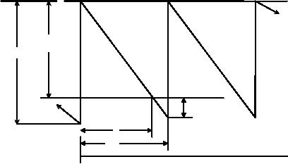
model is illustrated in Fig
.3
Im
Q
s
t1
t2
t
T
Fig.
3
Fig.
3 shows that the back
ordering is possible (i.e.)
once an order is received,
any shortages can be
made
up
as the items are received.
Consequently shortage costs
are due to being short of
stock for a period of
time.
The
cost per period includes
four cost components.
Total
cost per period = Item
cost + Order cost + Holding
cost + Shortage cost
Item
cost per period = (item
cost) �
(number
of items/period)
=
C1Q
(13)
Order
cost per period = C2
Let
t1 be the
time period during which
only the items are
held in stock. Let the
maximum inventory be denoted by
Im
and
this is equal to (Q
S)
or Im = (Q
S)
From
similar triangle concept,
the following equations can
be obtained, referring to fig
3
58

Operations
Research (MTH601)
59
t1 Im =
t
Q
(16)
Q
=
t
(Q -
S
)
/ Q
t
=tI
(17)
or
m
1
t2 S
=
t
Q
t
=tS
Q
(18)
or
2
Since
time of one period t =
Q
/
D
Q-S
Q
t =
(19)
QD
1
SQ
t =
(20)
QD
2
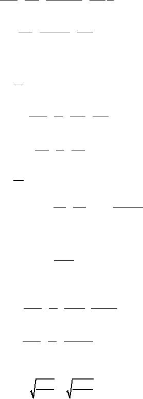
Holding
cost per period
=
Average
stock/period �
t1 �
hotlding
cost/unit/unit time
=
Im / 2
�
t1 �
C3
=
C3 �
(Q-S )
2 �
(Q-S )
Q
� Q
D
2
C3 (Q
-
S
)
=
(21)
2D
Shortage
cost per period
Average
shortages/period �
t2 �
shortage
cost
=
S
2
�
S Q � Q
D �
C4
=
C4 �
S 2 2D
(22)
Adding
all the four cost
components, we get the
inventory cost per
period.
C3 (Q-S )2 C4S
2
C′
= C1Q
+
C2 +
+
(23)
2D
2D
Therefore
inventory cost per unit of
time is obtained by dividing
C
′
bye
t
or Q/D
Therefore,
59

Operations
Research (MTH601)
60
C1QD
C 2D
C3 (Q-S )2 D C4S
2 D
C=
+
+
+
2D�Q
Q
Q
2D
Q
C2D
C3 (Q-S )2 C4S
2
=C D
+
+
+
(24)
Q
2Q
2Q
1
This
is an expression involving two
variables Q
and
S. For
optimum values of Q*
and
S*, the
function has to be
differentiated
partially with respect to
Q
and
S
and
equated to zero.
∂C
=0
∂Q
C3 C3S
2 C4S
2
-C2D
=
+
-
-
2
Q2
2
2Q2
2Q
S2
C2D
C3
=-
+
-
(C +
C
)
(25)
Q
2
2Q2
3
4
∂C
=0
∂S
S
(C3 +C4 )
C3S
C4S
=-C +
+
=
-C
+
(26)
Q
Q
Q
3
3
Solving
the equation (26) for
S, we
get
C3Q
S=
(27)
C3 +C4
Substituting
the equation (27) into
the equation (25), we
get
C3 C3 +C4 (C3 +Q)2
-C2D
0=
+
-
�
(28)
(C3 +C4 )
2
Q2
2Q2
2
-C2D
C3
C3
=
+
-
(29)
2
2(C3 +C4 )
Q2
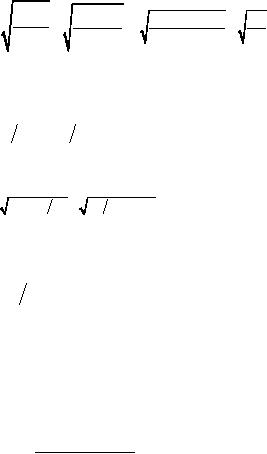
Solving
equation (29) for Q, we
get
C3 +C4
2C2D
Q*
=
(30)
C3
C4
60
Operations
Research (MTH601)
61
which
is the economic or optimum
order quantity.
2C2D
C3
S*
=
(31)
C3 +C4
C4
61

Operations
Research (MTH601)
62
Example:
The demand for an item is
18000 units/year. The cost
of one purchase is Rs. 400.
The holding cost is
Rs.
1.2
per unit per year.
The item cost is Rs. 1
per item. The shortage
cost is Rs. 5 per unit
per year. Determine:
(a)
The
optimum order
quantity.
(b)
The
time between orders.
(c)
The
number of orders per
year.
(d)
The
optimum shortages.
(e)
The
maximum inventory.
(f)
The
time of items being
held.
(g)
The
optimum annual cost.
Solution
D
= 18000
units/year
or
1500
units/month
C1 = Rs.
1/item
C3 = Rs.
1.2/year/item
C2 = Rs.
400/order
C4 = Rs.
5/year/item
C3 +
C4
2C
D
2�400�18000
6.2
=
2
Q*
=
�
a)
1.2
5
C4
C3
=
3857
Units.
t
*
+
Q*
D
=
3857
1500 =
2.57
months
b)
c)
Number
of orders per year = 12/2.57
= 4.66
S*
=
C3 (C3 +C4 ) =
747
items
d)
2C2 D
C4
=
Q
*
-S*
=
3857
-
747
=
3110
items
e)
I
max
D
=
3110
/ 1500 =
2.07
months
t
=I
f)
1
max
g)
Annual
cost = Item cost
+
Ordering cost
+
Holding cost
+
Shortage cost
Item
cost = Rs. 3857 per
order
Order
cost = Rs. 400 per
order
Rs.1.2�3110�2.07
=
Holding
cost
2�12
=
Rs.
322.14 per order
62
Table of Contents:
- Introduction:OR APPROACH TO PROBLEM SOLVING, Observation
- Introduction:Model Solution, Implementation of Results
- Introduction:USES OF OPERATIONS RESEARCH, Marketing, Personnel
- PERT / CPM:CONCEPT OF NETWORK, RULES FOR CONSTRUCTION OF NETWORK
- PERT / CPM:DUMMY ACTIVITIES, TO FIND THE CRITICAL PATH
- PERT / CPM:ALGORITHM FOR CRITICAL PATH, Free Slack
- PERT / CPM:Expected length of a critical path, Expected time and Critical path
- PERT / CPM:Expected time and Critical path
- PERT / CPM:RESOURCE SCHEDULING IN NETWORK
- PERT / CPM:Exercises
- Inventory Control:INVENTORY COSTS, INVENTORY MODELS (E.O.Q. MODELS)
- Inventory Control:Purchasing model with shortages
- Inventory Control:Manufacturing model with no shortages
- Inventory Control:Manufacturing model with shortages
- Inventory Control:ORDER QUANTITY WITH PRICE-BREAK
- Inventory Control:SOME DEFINITIONS, Computation of Safety Stock
- Linear Programming:Formulation of the Linear Programming Problem
- Linear Programming:Formulation of the Linear Programming Problem, Decision Variables
- Linear Programming:Model Constraints, Ingredients Mixing
- Linear Programming:VITAMIN CONTRIBUTION, Decision Variables
- Linear Programming:LINEAR PROGRAMMING PROBLEM
- Linear Programming:LIMITATIONS OF LINEAR PROGRAMMING
- Linear Programming:SOLUTION TO LINEAR PROGRAMMING PROBLEMS
- Linear Programming:SIMPLEX METHOD, Simplex Procedure
- Linear Programming:PRESENTATION IN TABULAR FORM - (SIMPLEX TABLE)
- Linear Programming:ARTIFICIAL VARIABLE TECHNIQUE
- Linear Programming:The Two Phase Method, First Iteration
- Linear Programming:VARIANTS OF THE SIMPLEX METHOD
- Linear Programming:Tie for the Leaving Basic Variable (Degeneracy)
- Linear Programming:Multiple or Alternative optimal Solutions
- Transportation Problems:TRANSPORTATION MODEL, Distribution centers
- Transportation Problems:FINDING AN INITIAL BASIC FEASIBLE SOLUTION
- Transportation Problems:MOVING TOWARDS OPTIMALITY
- Transportation Problems:DEGENERACY, Destination
- Transportation Problems:REVIEW QUESTIONS
- Assignment Problems:MATHEMATICAL FORMULATION OF THE PROBLEM
- Assignment Problems:SOLUTION OF AN ASSIGNMENT PROBLEM
- Queuing Theory:DEFINITION OF TERMS IN QUEUEING MODEL
- Queuing Theory:SINGLE-CHANNEL INFINITE-POPULATION MODEL
- Replacement Models:REPLACEMENT OF ITEMS WITH GRADUAL DETERIORATION
- Replacement Models:ITEMS DETERIORATING WITH TIME VALUE OF MONEY
- Dynamic Programming:FEATURES CHARECTERIZING DYNAMIC PROGRAMMING PROBLEMS
- Dynamic Programming:Analysis of the Result, One Stage Problem
- Miscellaneous:SEQUENCING, PROCESSING n JOBS THROUGH TWO MACHINES
- Miscellaneous:METHODS OF INTEGER PROGRAMMING SOLUTION