THE RELATIVE FREQUENCY DEFINITION OF PROBABILITY:INDEPENDENT EVENTS

<< THE RELATIVE FREQUENCY DEFINITION OF PROBABILITY:ADDITION LAW

MTH001 Elementary Mathematics

LECTURE # 32:

· Independent and Dependent Events

· Multiplication Theorem of Probability for Independent Events

· Marginal Probability

Before we proceed the concept of independent versus dependent events, let us review the

Addition and Multiplication Theorems of Probability that were discussed in the last lecture.

To this end, let us consider an interesting example that illustrates the application of both of

these theorems in one problem:

EXAMPLE:

A bag contains 10 white and 3 black balls. Another bag contains 3 white and 5 black balls.

Two balls are transferred from first bag and placed in the second, and then one ball is taken

from the latter.

What is the probability that it is a white ball?

In the beginning of the experiment, we have:

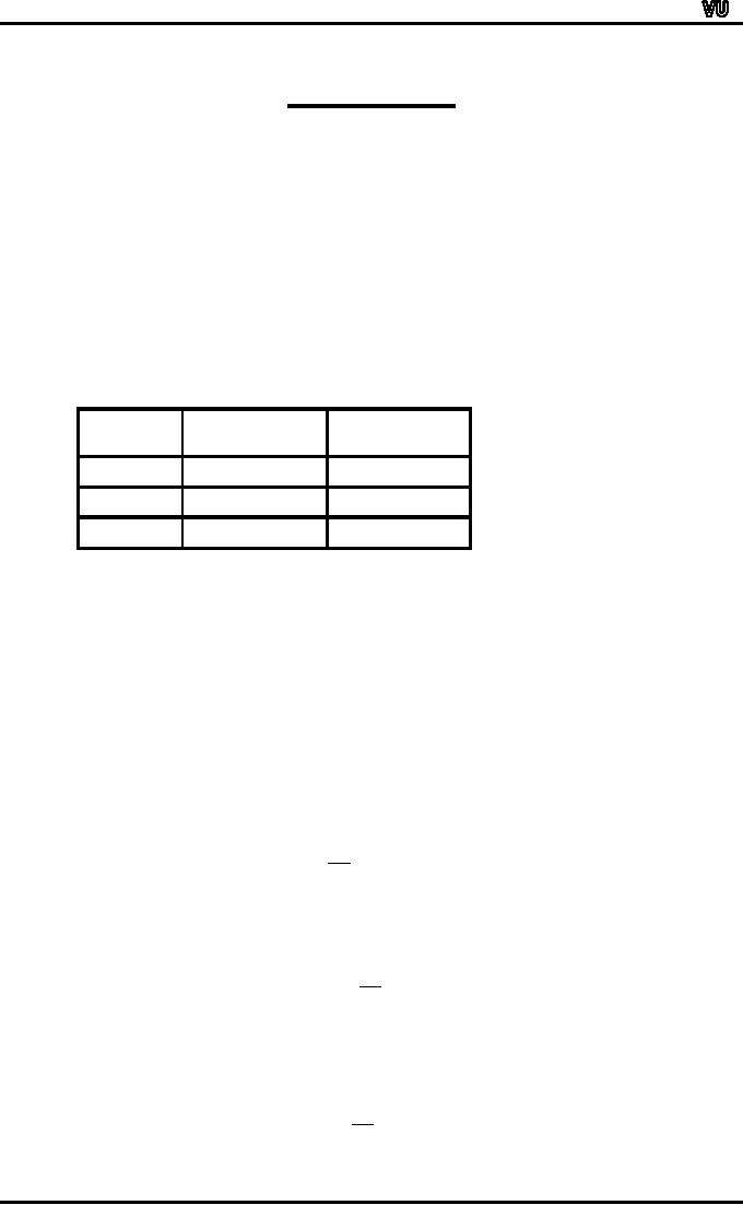
Colour of

No. of

Ball

Balls in Bag A

Balls in Bag B

White

Black

Total

Let A represent the event that 2 balls are drawn from the first bag and transferred to the

second bag. Then A can occur in the following three mutually exclusive ways:

A1 = 2 white balls are transferred to the second bag.

A2 = 1 white ball and 1 black ball are transferred to the second bag. ⎛13⎞

⎜ ⎟.

⎜ 2⎟

A3 = 2 black balls are transferred to the second bag.

⎝ ⎠

Then, the total number of ways in which 2 balls can be drawn out of a total of 13 balls is ⎛10 ⎞

⎜ ⎟.

⎜ 2⎟

⎝ ⎠

And, the total number of ways in which 2 white balls can be drawn out of 10 white balls is

Thus, the probability that two white balls are selected from the first bag containing 13 balls

(in order to transfer to the second bag) is

⎛10 ⎞ ⎛13⎞ 45

P( A1 ) = ⎜ ⎟ ÷ ⎜ ⎟ =

⎜ 2 ⎟ ⎜ 2 ⎟ 78 ,

⎝ ⎠ ⎝ ⎠

Similarly, the probability that one white ball and one black ball are selected from the first bag

containing 13 balls (in order to transfer to the second bag) is

⎛10 ⎞ ⎛ 3⎞ ⎛13⎞ 30

P( A2 ) = ⎜ ⎟ ⎜ ⎟ ÷ ⎜ ⎟ = ,

⎜ 1 ⎟ ⎜1 ⎟ ⎜ 2 ⎟ 78

⎝ ⎠⎝ ⎠ ⎝ ⎠

And, the probability that two black balls are selected from the first bag containing 13 balls (in

order to transfer to the second bag) is

⎛ 3 ⎞ ⎛13⎞ 3

P( A3 ) = ⎜ ⎟ ÷ ⎜ ⎟ = .

⎜ 2 ⎟ ⎜ 2 ⎟ 78

⎝ ⎠ ⎝ ⎠

Page

222

MTH001 Elementary Mathematics

AFTER having transferred 2 balls from the first bag, the second bag contains

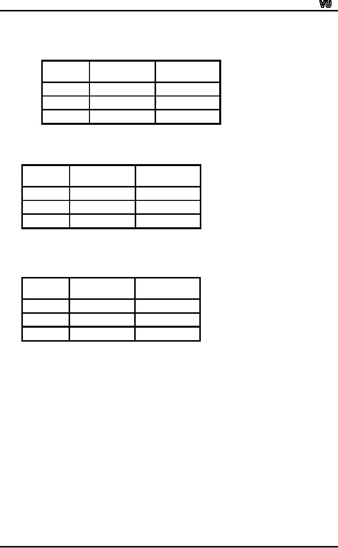
i) 5 white and 5 black balls (if 2 white balls are transferred)

Colour of

No. of

Ball

Balls in Bag A

Balls in Bag B

White

10 2 = 8

3+2=5

Black

Total

13 2 = 11

8 + 2 = 10

Hence: P(W/A1) = 5/10

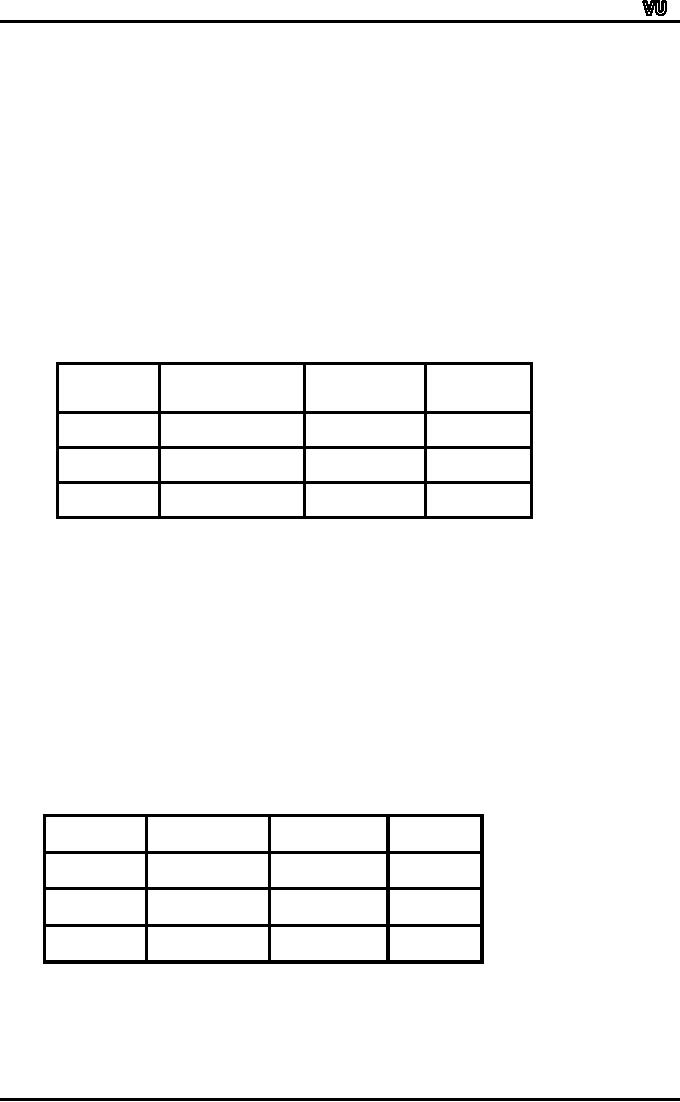
ii)

4 white and 6 black balls

(if 1 white and 1 black ball are transferred)

Colour of

No. of

Ball

Balls in Bag A

Balls in Bag B

White

10 1 = 7

3+1=4

Black

31=2

5+1=4

Total

13 2 = 11

8 + 2 = 10

Hence: P(W/A2) = 4/10

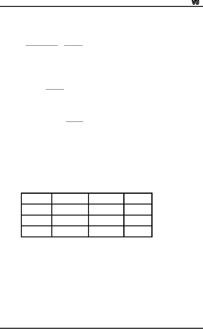
iii)

3 white and 7 black balls

(if 2 black balls are transferred)

Colour of

No. of

Ball

Balls in Bag A

Balls in Bag B

White

Black

32=1

5+2=7

Total

13 2 = 11

8 + 2 = 10

Hence: P(W/A3) = 3/10

Let W represent the event that the WHITE ball is drawn from the second bag after

having transferred 2 balls from the first bag.

Then P(W) = P(A1∩W) + P(A2∩W) + P(A3∩W)

Now P(A1 ∩ W) = P(A1)P(W/A1)

= 45/78 × 5/10

= 15/52

P(A2 ∩ W) = P(A2)P(W/A2)

= 30/78 × 4/10

= 2/13,

and

P(A3 ∩ W) = P(A3)P(W/A3)

= 3/78 × 3/10

= 3/260.

Hence the required probability is

P(W)

= P(A1∩W) + P(A2∩W) + P(A3∩W)

Page

223

MTH001 Elementary Mathematics

= 15/52 + 2/13 + 3/260

= 59/130

= 0.45

Next, we discuss the concept of INDEPENDENT EVENTS:

INDEPENDENT EVENTS:

Two events A and B in the same sample space S, are defined to be independent (or

statistically independent) if the probability that one event occurs, is not affected by whether

the other event has or has not occurred, that is

P(A/B) = P(A) and P(B/A) = P(B).

It then follows that two events A and B are independent if and only if

P(A ∩ B) = P(A) P(B)

and this is known as the special case of the Multiplication Theorem of Probability.

RATIONALE:

According to the multiplication theorem of probability, we have:

P(A ∩ B) = P(A) . P(B/A)

Putting P(B/A) = P(B), we obtain

P(A ∩ B) = P(A) P(B)

The events A and B are defined to be DEPENDENT if P(A∩B) ≠ P(A) × P(B).

This means that the occurrence of one of the events in some way affects the probability of

the occurrence of the other event. Speaking of independent events, it is to be emphasized

that two events that are independent, can NEVER be mutually exclusive.

EXAMPLE:

Two fair dice, one red and one green, are thrown.

Let A denote the event that the red die shows an even number and let B denote the event

that the green die shows a 5 or a 6. Show that the events A and B are independent.

The sample space S is represented by the following 36 outcomes:

S = {(1, 1), (1, 2), (1, 3), (1, 5), (1, 6);

(2, 1), (2, 2), (2, 3), (2, 5), (2, 6);

(3, 1), (3, 2), (3, 3), (3, 5), (3, 6);

(4, 1), (4, 2), (4, 3), (4, 5), (4, 6);

(5, 1), (5, 2), (5, 3), (5, 5), (5, 6);

(6, 1), (6, 2), (6, 3), (6, 5), (6, 6) }

Since

A represents the event that red die shows an even number, and B represents the event that

green die shows a 5 or a 6,

Therefore A ∩ B represents the event that red die shows an even number and green die

shows a 5 or a 6.

Since A represents the event that red die shows an even number, hence P(A) = 3/6.

Similarly, since B represents the event that green die shows a 5 or a 6, hence P(B) = 2/6.

Now, in order to compute the probability of the joint event A ∩ B, the first point to

note is that, in all, there are 36 possible outcomes when we throw the two dice together, i.e.

S = {(1, 1), (1, 2), (1, 3), (1, 5), (1, 6);

(2, 1), (2, 2), (2, 3), (2, 5), (2, 6);

(3, 1), (3, 2), (3, 3), (3, 5), (3, 6);

(4, 1), (4, 2), (4, 3), (4, 5), (4, 6);

(5, 1), (5, 2), (5, 3), (5, 5), (5, 6);

(6, 1), (6, 2), (6, 3), (6, 5), (6, 6) }

The joint event A ∩ B contains only 6 outcomes out of the 36 possible outcomes.

These are (2, 5), (4, 5), (6, 5), (2, 6), (4, 6), and (6, 6).

P(A ∩ B) = 6/36.

and

Now

P(A) P(B)

Page

224

MTH001 Elementary Mathematics

= 3/6 × 2/6

= 6/36

= P(A ∩ B).

Therefore the events A and B are independent.

Let us now go back to the example pertaining to live births and stillbirths that we

considered in the last lecture, and try to determine whether or not sex of the baby and

nature of birth are independent.

EXAMPLE :

Table-1 below shows the numbers of births in England and Wales in 1956 classified

by (a) sex and (b) whether live born or stillborn.

Table-1

Number of births in England and Wales in 1956 by sex and whether live- or still born.

(Source Annual Statistical Review)

Liveborn

Stillborn

Total

Male

359,881 (A)

8,609 (B)

368,490

Female 340,454 (B)

7,796 (D)

348,250

Total

700,335

16,405

716,740

There are four possible events in this double classification:

· Male live birth,

· Male stillbirth,

· Female live birth, and

· Female stillbirth.

The corresponding relative frequencies are given in Table-2.

Table-2

Proportion of births in England and Wales in 1956 by sex and whether live- or stillborn.

(Source Annual Statistical Review)

Liveborn

Stillborn

Total

Male

.5021

.0120

.5141

Female

.4750

.0109

.4859

Total

.9771

.0229

1.0000

As discussed in the last lecture, the total number of births is large enough for these relative

frequencies to be treated for all practical purposes as PROBABILITIES.

Page

225

MTH001 Elementary Mathematics

The compound events `Male birth' and `Stillbirth' may be represented by the letters M

and S.

If M represents a male birth and S a stillbirth, we find that

n(M and S )

8609

= 0.0234

n (M )

368490

This figure is the proportion and, since the sample size is large, it can be regarded as the

probability of males who are still born in other words, the CONDITIONAL probability of

a stillbirth given that it is a male birth. In other words, the probability of stillbirths in males.

The corresponding proportion of stillbirths among females is

7796

= 0.0224.

348258

These figures should be contrasted with the OVERALL, or UNCONDITIONAL, proportion of

stillbirths, which is

16405

= 0.0229.

716740

We observe that the conditional probability of stillbirths among boys is slightly HIGHER than

the overall proportion. Where as the conditional proportion of stillbirths among girls is slightly

LOWER than the overall proportion. It can be concluded that sex and stillbirth are

statistically DEPENDENT, that is to say, the SEX of a baby yet to be born has an effect,

(although a small effect), on its chance of being stillborn. The example that we just

considered point out the concept of MARGINAL PROBABILITY.

Let us have another look at the data regarding the live births and stillbirths in

England and Wales:

Table-2Proportion of births in England and Wales in 1956 by sex and whether live- or

stillborn. (Source Annual Statistical Review)

Liveborn

Stillborn

Total

Male

.5021

.0120

.5141

Female

.4750

.0109

.4859

Total

.9771

.0229

1.0000

And, the figures in Table-2 indicate that the probability of male birth is 0.5141, whereas the

probability of female birth is 0.4859.Also, the probability of live birth is 0.9771, where as the

probability of stillbirth is 0.0229.

And since these probabilities appear in the margins of the Table, they are known as

Marginal Probabilities. According to the above table, the probability that a new born baby is

a male and is live born is 0.5021 whereas the probability that a new born baby is a male and

is stillborn is 0.0120.Also, as stated earlier, the probability that a new born baby is a male is

0.5141, and, CLEARLY, 0.5141 = 0.5021 + 0.0120.

Hence, it is clear that the joint probabilities occurring in any row of the table ADD UP to yield

the corresponding marginal probability.

If we reflect upon this situation carefully, we will realize that this equation is totally in

accordance with the Addition Theorem of Probability for mutually exclusive events.

Page

226

MTH001 Elementary Mathematics

P(male birth)

= P(male live-born or male stillborn)

= P(male live-born) + P(male stillborn)

= 0.5021 + 0.0120

= 0.5141

Another important point to be noted is that:

Conditional Probability

Joint Probability

Marginal Probability

EXAMPLE:

P(stillbirth/male birth)

P(male birth and stillbirth)/P(male birth)

=0.0120/0.5141

= 0.0233

Page

227

Table of Contents: