THE RELATIVE FREQUENCY DEFINITION OF PROBABILITY:ADDITION LAW

<< Definitions of Probability:MUTUALLY EXCLUSIVE EVENTS, Venn Diagram

THE RELATIVE FREQUENCY DEFINITION OF PROBABILITY:INDEPENDENT EVENTS >>

MTH001 Elementary Mathematics

LECTURE # 31:

Relative Frequency Definition of Probability

Axiomatic Definition of Probability

Laws of Probability

· Rule of Complementation

· Addition Theorem

THE RELATIVE FREQUENCY DEFINITION OF PROBABILITY

(`A POSTERIORI' DEFINITION OF PROBABILITY):

If a random experiment is repeated a large number of times, say n times, under

identical conditions and if an event A is observed to occur m times, then the probability of

the event A is defined as the LIMIT of the relative frequency m/n as n tends to infinitely.

Symbolically, we write

P( A) = Lim

n→∞

The definition assumes that as n increases indefinitely, the ratio m/n tends to become stable

at the numerical value P(A). The relationship between relative frequency and probability can

also be represented as follows:

Relative Frequency → Probability

as n → ∞

As its name suggests, the relative frequency definition relates to the relative frequency with

which are event occurs in the long run. In situations where we can say that an experiment

has been repeated a very large number of times, the relative frequency definition can be

applied.

As such, this definition is very useful in those practical situations where we are

interested in computing a probability in numerical form but where the classical definition

cannot be applied.(Numerous real-life situations are such where various possible outcomes

of an experiment are NOT equally likely). This type of probability is also called empirical

probability as it is based on EMPIRICAL evidence i.e. on OBSERVATIONAL data.

It can also be called STATISTICAL PROBABILITY for it is this very probability that forms

the basis of mathematical statistics.

Let us try to understand this concept by means of two examples:

1) from a coin-tossing experiment and

2) from data on the numbers of boys and girls born.

EXAMPLE-1:

Coin-Tossing:

No one can tell which way a coin will fall but we expect the proportion of leads and tails after

a large no. of tosses to be nearly equal. An experiment to demonstrate this point was

performed by Kerrich in Denmark in 1946. He tossed a coin 10,000 times, and obtained

altogether 5067 heads and 4933 tails.

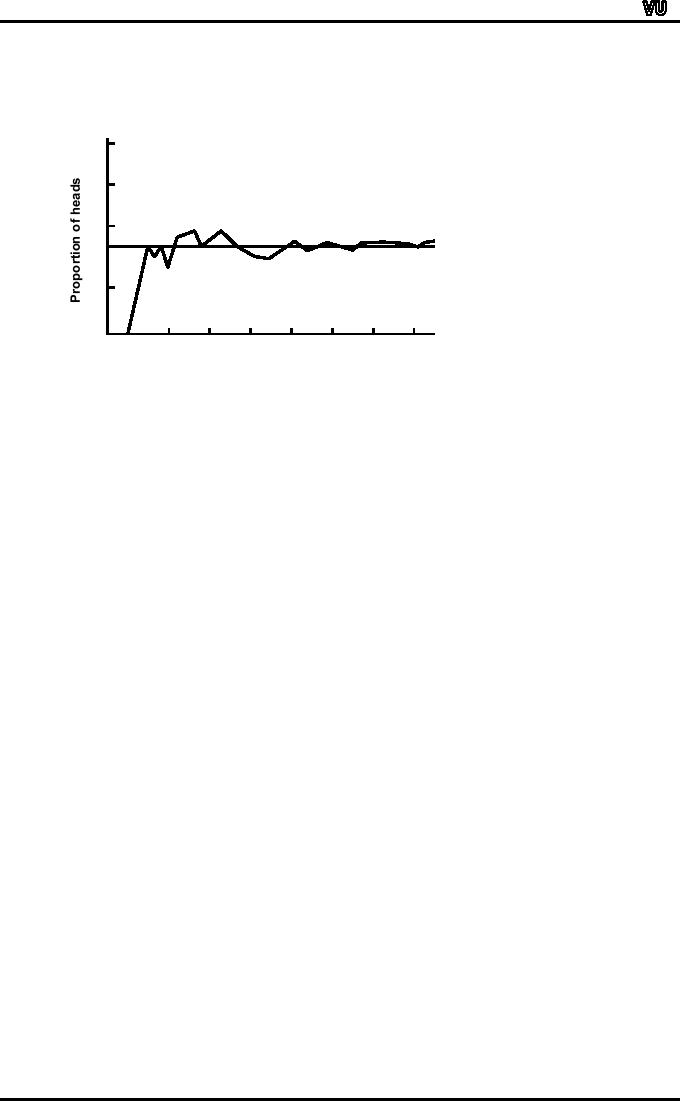
The behavior of the proportion of heads throughout the experiment is shown as in the

following figure:

Page

216

MTH001 Elementary Mathematics

The proportion; of heads in a sequence of tosses of a coin (Kerrich, 1946):

1.0

100

300

1000

3000

10000

Number of tosses (logarithmic scale)

As you can see, the curve fluctuates widely at first, but begins to settle down to a more or

less stable value as the number of spins increases. It seems reasonable to suppose that the

fluctuations would continue to diminish if the experiment were continued indefinitely, and the

proportion of heads would cluster more and more closely about a limiting value which would

be very near, if not exactly, one-half.

This hypothetical limiting value is the (statistical) probability of heads.

Let us now take an example closely related to our daily lives --- that relating to the sex ratio:-

In this context, the first point to note is that it has been known since the eighteenth century

that in reliable birth statistics based on sufficiently large numbers (in at least some parts of

the world), there is always a slight excess of boys,

Laplace records that, among the 215,599 births in thirty districts of France in the years 1800

to 1802, there were 110,312 boys and 105,287 girls.

The proportions of boys and girls were thus 0.512 and 0.488 respectively (indicating a slight

excess of boys over girls).In a smaller number of births one would, however, expect

considerable deviations from these proportions.

This point can be illustrated with the help of the following example:

EXAMPLE-2:

The following table shows the proportions of male births that have been worked out for the

major regions of England as well as the rural districts of Dorset (for the year 1956):

Page

217

MTH001 Elementary Mathematics

Proportions of Male Births in various Regions

and Rural Districts of England in 1956

(Source: Annual Statistical Review)

Propo rtio n

Region of

Rura l Districts of

of Ma le

Eng land

Do rset

Births

No rthern

.514

Beaminste r

.38

E. & W. Riding

.513

Blandfo rd

.47

No rth Weste rn

.512

Bridpo rt

.53

No rth Midland

.517

Do rcheste r

.50

Midland

.514

Shaftesbury

.59

Eastern

.516

She rbo rne

.44

London and S.

.514

Sturminste r

.54

Eastern

Wa re ham and

Southe rn

.514

.53

Purbeck

Wimbo rne &

South Weste rn

.513

.54

Cranbo rne

All Rura l District's

Who le country

.514

.512

of Do rset

As you can see, the figures for the rural districts of Dorset, based on about 200 births each,

fluctuate between 0.38 and 0.59. While those for the major regions of England, which are

each based on about 100,000 births, do not fluctuate much, rather, they range between

0.512 and 0.517 only. The larger sample size is clearly the reason for the greater constancy

of the latter. We can imagine that if the sample were increased indefinitely, the proportion of

boys would tend to a limiting value which is unlikely to differ much from 0.514, the proportion

of male births for the whole country.

This hypothetical limiting value is the (statistical) probability of a male birth.

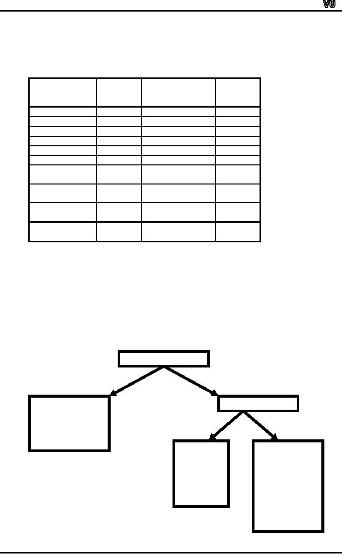
The overall discussion regarding the various ways in which probability can be defined is

presented in the following diagram:

Probability

Non-Quantifiable

Quantifiable

(Inductive,

Subjective or

Personalistic

Probability)

" A Priori "

Statistical

Probability

(Verifiable

(Empirical or

through

" A Posteriori "

Empirical

Probability)

↑

Evidence)

(A statistician's

main concern)

Page

218

MTH001 Elementary Mathematics

As far as quantifiable probability is concerned, in those situations where the various possible

outcomes of our experiment are equally likely, we can compute the probability prior to

actually conducting the experiment --- otherwise, as is generally the case, we can compute

a probability only after the experiment has been conducted (and this is why it is also called

`a posteriori' probability).

Non-quantifiable probability is the one that is called Inductive Probability.

It refers to the degree of belief which it is reasonable to place in a proposition on given

evidence.

An important point to be noted is that it is difficult to express inductive probabilities

numerically to construct a numerical scale of inductive probabilities, with 0 standing for

impossibility and for logical certainty. An important point to be noted is that it is difficult to

express inductive probabilities numerically to construct a numerical scale of inductive

probabilities, with 0 standing for impossibility and for logical certainty.

Most statisticians have arrived at the conclusion that inductive probability cannot, in general,

he measured and, therefore cannot be use in the mathematical theory of statistics.

This conclusion is not, perhaps, very surprising since there seems

no reason why rational degree of belief should be measurable any more than, say, degrees

of beauty. Some paintings are very beautiful, some are quite beautiful, and some are ugly,

but it would be observed to try to construct a numerical scale of beauty, on which Mona Lisa

had a beauty value of 0.96.Similarly some propositions are highly probable, some are quite

probable and some are improbable, but it does not seem possible to construct a numerical

scale of such (inductive) probabilities .Because of the fact that inductive probabilities are not

quantifiable and cannot be employed in a mathematical argument, this is the reason why the

usual methods of statistical inference such as tests of significance and confidence interval

are based entirely on the concept of statistical probability. Although we have discussed

three different ways of defining probability, the most formal definition is yet to come.

This is The Axiomatic Definition of Probability.

THE AXIOMATIC DEFINITION OF PROBABILITY:

This definition, introduced in 1933 by the Russian mathematician

Andrei N. Kolmogrov, is based on a set of AXIOMS.

Let S be a sample space with the sample points E1, E2, ... Ei, ...En. To each sample point,

we assign a real number, denoted by the symbol P(Ei), and called the probability of Ei, that

must satisfy the following basic axioms:

Axiom 1:

For any event Ei,

0 < P(Ei) < 1.

Axiom 2:

P(S) =1

for the sure event S.

Axiom 3:

If A and B are mutually exclusive events (subsets of S), then

P (A ∪ B) = P(A) + P(B).

It is to be emphasized that According to the axiomatic theory of probability:

SOME probability defined as a non-negative real number is to be ATTACHED to each

sample point Ei such that the sum of all such numbers must equal ONE.

The ASSIGNMENT of probabilities may be based on past evidence or on some other

underlying conditions.

Page

219

MTH001 Elementary Mathematics

(If this assignment of probabilities is based on past evidence, we are talking about

EMPIRICAL probability, and if this assignment is based on underlying conditions that ensure

that the various possible outcomes of a random experiment are EQUALLY LIKELY, then we

are talking about the CLASSICAL definition of probability.

Let us consider another example:

EXAMPLE :

Table-1

below shows the numbers of births in England and Wales in 1956 classified by (a) sex

and (b) whether liveborn or stillborn.

Table-1

Number of births in England and Wales in 1956 by sex and whether live- or still born.

(Source Annual Statistical Review)

Livebo rn

Stillbo rn

Tota l

Ma le

359,881 (A)

8,609 (B )

368,490

F emale

340,454 (B )

7,796 (D)

348,250

Tota l

700,335

16,405

716,740

There are four possible events in this double classification:

· Male livebirth (denoted by A),

· Male stillbirth (denoted by B),

· Female livebirth (denoted by C)

and

· Female stillbirth (denoted by D),

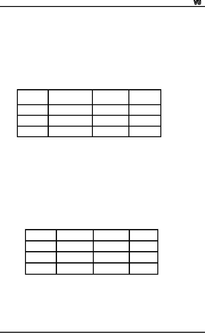
The relative frequencies corresponding to the figures of Table-1 are given in Table-2:

Table-2

Proportion of births in England and Wales in 1956 by sex and whether live- or

stillborn.

(Source Annual Statistical Review)

Livebo rn

Stillbo rn

Tota l

Ma le

.5021

.0120

.5141

F emale

.4750

.0109

.4859

Tota l

.9771

.0229

1.0000

The total number of births is large enough for these relative frequencies to be treated for all

practical purposes as PROBABILITIES.

Let us denote the compound events `Male birth' and `Stillbirth' by the letters M

and S.Now a male birth occurs whenever either a male livebirth or a male stillbirth occurs,

Page

220

MTH001 Elementary Mathematics

and so the proportion of male birth, regardless of whether they are live-or stillborn, is equal

to the sum of the proportions of these two types of birth; that is to say,

p(M)

= p(A or B) = p(A) + p(B)

= .5021 + .0120 = .5141

Similarly, a stillbirth occurs whenever either a male stillbirth or a female stillbirth occurs and

so the proportion of stillbirths, regardless of sex, is equal to the sum of the proportions of

these two events:

p(S)

= p(B or D) = p(B) + p(D)

= .0120 + .0109 = .0229.

Let us now consider some basic LAWS of probability.

These laws have important applications in solving probability problems.

LAW OF COMPLEMENTATION:

If ⎯A is the complement of an event A relative to the sample space S, then

P(A ) = 1 - P( A).

Hence the probability of the complement of an event is equal to one minus the probability of

the event.

Complementary probabilities are very useful when we are wanting to solve

questions of the type `What is the probability that, in tossing two fair dice, at least one even

number will appear?'

EXAMPLE:

A coin is tossed 4 times in succession. What is the probability that at least one head occurs?

(1) The sample space S for this experiment consists of 24 = 16 sample points (as each toss

can result in 2 outcomes),and

(2) we assume that each outcome is equally likely.

If we let A represent the event that at least one head occurs, then A will consist

of MANY sample points, and the process of computing the probability of this event will

become somewhat cumbersome! So, instead of denoting this particular event by A, let us

denote its complement i.e. "No head" by A.

Thus the event A consists of the SINGLE sample point {TTTT}.

Therefore P(A ) = 1/16.

Hence by the law of complementation, we have

P(A ) = 1 - P(A ) = 1 -

1 15

= .

16 16

The next law that we will consider is the Addition Law or the General Addition Theorem of

Probability:

ADDITION LAW:

If A and B are any two events defined in a sample space S, then

P(A∪B) = P(A) + P(B) P(A∩B)

In words, this law may be stated as follows:

"If two events A and B are not mutually exclusive, then the probability that at

least one of them occurs, is given by the sum of the separate probabilities of events A and

B minus the probability of the joint event A ∩ B."

Page

221

Table of Contents: