 |
GEOMETRIC MEAN:HARMONIC MEAN, MID-QUARTILE RANGE |
| << Median in Case of a Frequency Distribution of a Continuous Variable |
| GEOMETRIC MEAN:Number of Pupils, QUARTILE DEVIATION: >> |
MTH001
Elementary Mathematics
LECTURE #
26:
� Geometric
mean
� Harmonic
mean
� Relation
between the arithmetic,
geometric and harmonic
means
�
Some
other measures of central
tendency
GEOMETRIC
MEAN:
The
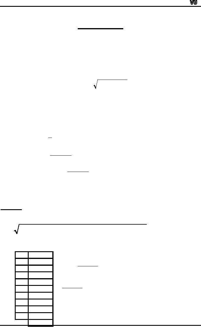
geometric mean, G, of a set of n
positive values X1, X2,...,Xn is
defined as the
positive
nth
root of their
product.
G
=
n
X 1 X
2 ...X
n
(Where
Xi >
0)
When
n is large, the computation of
the geometric mean becomes
laborious as we have to
extract
the nth root of the
product of all the
values.
The
arithmetic is simplified by the
use of logarithms.
Taking
logarithms to the base 10,
we get
1
[log
X1 +
log
X
2 +
....+ log
X
n ]
log
G
=
n
∑
log
X
=
Hence
n
⎡
∑ log
X ⎤
G
=
anti
log ⎢
⎥
⎦
⎣ n
Example:
Find
the geometric mean of
numbers:
45,
32, 37, 46,
39,
36,
41, 48, 36.
Solution:
We
need to compute the
numerical value of
9
45� 32�
37
�
46�
39�
36�
41�
48�
36
=
But,
obviously, it is a bit cumbersome to
find the ninth root of a
quantity. So we make use
of
logarithms,
as shown below:
X
log
X
∑
log
X
45
1.6532
log
G =
32
1.5052
n
37
1.5682
46
1.6628
14.3870
=
=
1.5986
39
1.5911
9
36
1.5563
41
1.6128
Hence
G =
anti
log 1.5986
48
1.6812
=
39.68
36
1.5563
14.3870
Page
181
MTH001
Elementary Mathematics
The
above example pertained to
the computation of the
geometric mean in case of
raw
data.
Next,
we consider the computation of
the geometric mean in the
case of grouped data.
GEOMETRICMEAN
FOR
GROUPED DATA:
In
case of a frequency distribution
having k classes with
midpoints X1, X2,
...,Xk
and the corresponding
frequencies f1, f2, ..., fk
(such that ∑fi = n),
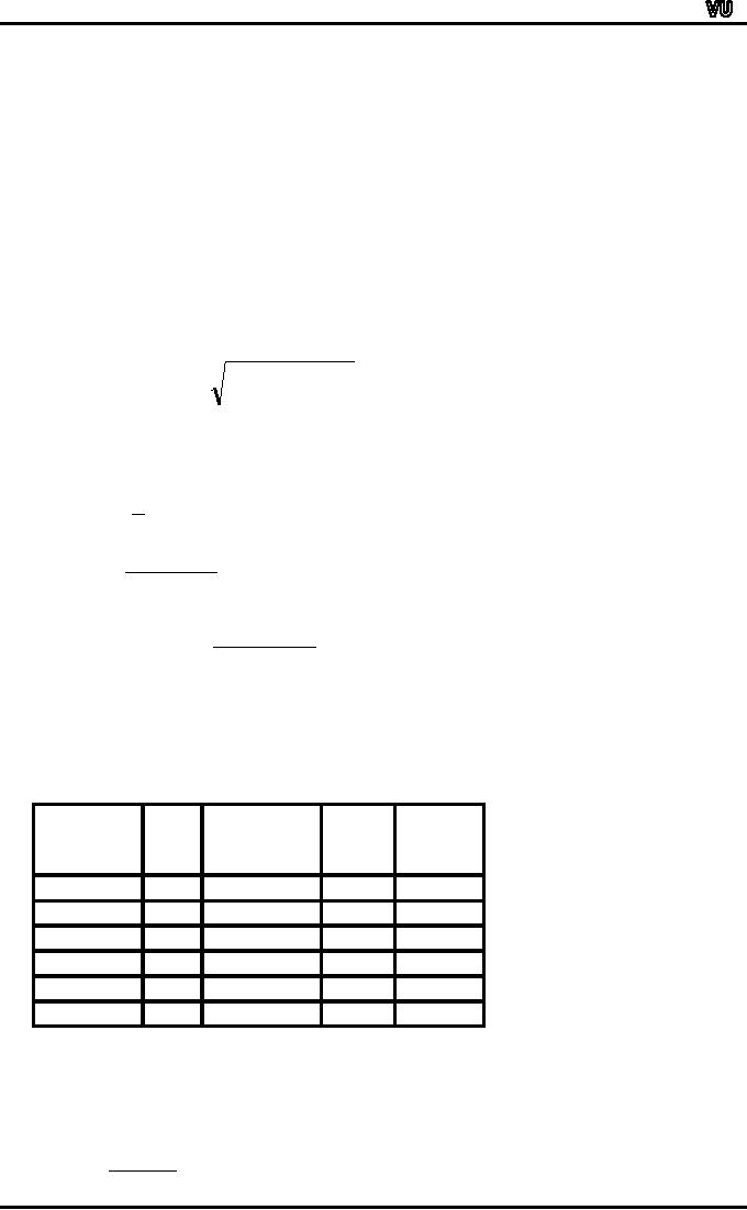
the geometric
mean
is given by
G
=
X11
Xf2
....Xfk
f
n
2
k
Each
value of X thus has to be
multiplied by itself f times,
and the whole procedure
becomes
quite
a formidable task!
In
terms of logarithms, the
formula becomes
1
[
f1 log X
1 +
f
2 log X
2 +
...
+
f
k log
X
k ]
log
G
=
n
∑
f
log
X
=
n
Hence
⎡∑f
log
X
⎤
G
=
anti
og⎢
l
⎥
n
⎢
⎥
⎣
⎦
Obviously,
the above formula is much
easier to handle.
Let
us now apply it to an
example.
Going
back to the example of the
EPA mileage ratings, we
have:
No.
Class-mark
Mileage
log
X
f
log X
of
(midpoint)
Rating
Cars
X
30.0
- 32.9
2
31.45
1.4976
2.9952
33.0
- 35.9
4
34.45
1.5372
6.1488
36.0
- 38.9
14
37.45
1.5735
22.0290
39.0
- 41.9
8
40.45
1.6069
12.8552
42.0
- 44.9
2
43.45
1.6380
3.2760
30
47.3042
G
= antilog
47.3042
30
Page
182
MTH001
Elementary Mathematics
=
antilog 1.5768 =
37.74
This
means that, if we use the
geometric mean to measures
the central tendency of
this
data
set, then the central
value of the mileage of
those 30 cars comes out to
be 37.74 miles
per
gallon.
The
question is, "When should we
use the geometric
mean?"
The
answer to this question is
that when relative changes
in some variable quantity
are
averaged,
we prefer the geometric
mean.
EXAMPLE:
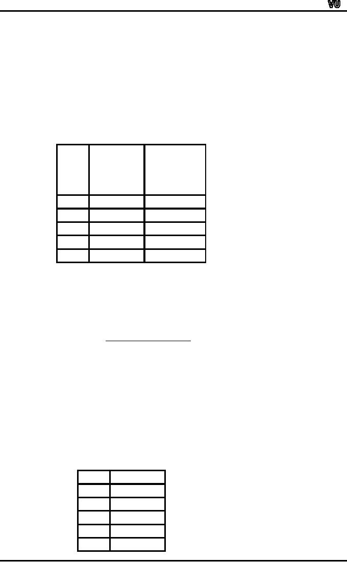
Suppose
it is discovered that a firm's
turnover has increased
during 4 years by the
following
amounts:
Percentage
Compared
Year
Turnover
With
Year
Earlier
1958
�
2,000
1959
�
2,500
125
1960
�
5,000
200
1961
�
7,500
150
1962
�
10,500
140
The
yearly increase is shown in a
percentage form in the
right-hand column i.e. the
turnover
of
1959 is 125 percent of the
turnover of 1958, the
turnover of 1960 is 200
percent of the
turnover
of 1959, and so on. The
firm's owner may be
interested in knowing his
average rate
of
turnover growth.
If
the arithmetic mean is
adopted he finds his answer
to be:
Arithmetic
Mean:
125
+
200
+
150
+
140
4
=
153.75
i.e.
we are concluding that the
turnover for any year is
153.75% of the turnover for
the
previous
year. In other words, the
turnover in each of the
years considered appears to
be
53.75
per cent higher than in
the previous year.
If
this
percentage is
used to calculate the
turnover from 1958 to 1962
inclusive, we obtain:
153.75%
of � 2,000 = � 3,075
153.75%
of � 3,075 = � 4,728
153.75%
of � 4,728 = � 7,269
153.75%
of � 7,269 = � 11,176
Whereas
the actual turnover figures
were
Year
Turnover
1958
�
2,000
1959
�
2,500
1960
�
5,000
1961
�
7,500
1962
� 10,500
Page
183

MTH001
Elementary Mathematics
It
seems that both the
individual figures and, more
important, the total at the
end of the
period,
are incorrect. Using the
arithmetic mean has
exaggerated the `average'
annual rate
of
increase in the turnover of
this firm. Obviously, we
would like to rectify this
false
impression.
The geometric mean enables
us to do so:
Geometric
mean of the turnover
figures:
(125
�
200
�150
�140)
4
4
=
525000000
=
151.37%
Now,
if we utilize this particular
value to obtain the
individual turnover figures, we
find that:
151.37%
of �2,000 = �3,027
151.37%
of �3,027 = �4,583
151.37%
of �4,583 = �6,937
151.37%
of �6,937 = �10,500
So
that the turnover figure of
1962 is exactly the same as
what we had in the original
data.
Interpretation:
If
the turnover of this company
were to increase annually at a
constant rate, then the
annual
increase
would have been 51.37
percent.(On the average,
each year's turnover is
51.37%
higher
than that in the previous
year.) The above example
clearly indicates the
significance
of
the geometric mean in a
situation when relative
changes in a variable quantity
are to be
averaged.
But
we should bear in mind that
such situations are not
encountered too often,
and
that
the occasion to calculate
the geometric mean arises
less frequently than the
arithmetic
mean.(The
most frequently used measure
of central tendency is the
arithmetic mean.)
The
next measure of central
tendency that we will
discuss is the harmonic
mean.
HARMONIC
MEAN;
The
harmonic mean is defined as
the reciprocal of the
arithmetic mean of
the
reciprocals
of the values. HARMONIC
MEAN
In
case of raw data:
n
H
.M .
=
⎛1⎞
∑⎜ X
⎟
⎝ ⎠
In
case of grouped data (data
grouped into a frequency
distribution):
n
H
.M .
=
⎛1⎞
∑
f⎜
⎟
⎝X⎠
(where
X represents the midpoints of
the various classes).
EXAMPLE:
Suppose
a car travels 100 miles
with 10 stops, each stop
after an interval of 10
miles.
Suppose that the speeds at
which the car travels
these 10 intervals are 30,
35, 40,
40,
45, 40, 50, 55, 55
and 30 miles per hours
respectively.
What
is the average speed with
which the car traveled
the total distance of 100
miles?
If
we find the arithmetic mean
of the 10 speeds, we
obtain:
Arithmetic
mean of the 10
speeds:
Page
184
MTH001
Elementary Mathematics
30
+
35
+
....
+
30
10
420
miles
per hour.
=
=
42
10
But,
if we study the problem
carefully, we find that the
above answer is
incorrect.
By
definition, the average
speed is the speed with
which the car
would
have traveled the 100
mile distance if it had
maintained a constant speed
throughout
the
10 intervals of 10 miles
each.
Total
distance travelled
Average
speed =
Total
time taken
Now,
total
distance traveled = 100
miles.
Total
time taken will be
computed as shown
below:
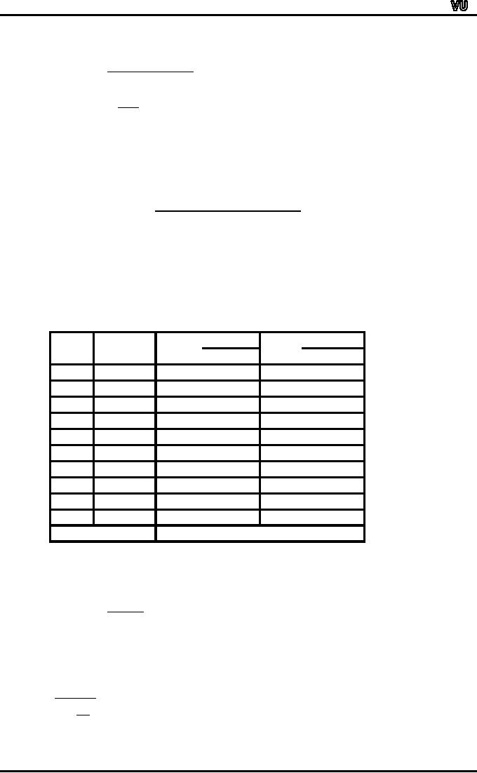
Distance
Distance
Interval
Distance
Speed
=
Time
=
Time
Speed
1
10
miles
30
mph
10/30
= 0.3333 hrs
2
10
miles
35
mph
10/35
= 0.2857 hrs
3
10
miles
40
mph
10/40
= 0.2500 hrs
4
10
miles
40
mph
10/40
= 0.2500 hrs
5
10
miles
45
mph
10/45
= 0.2222 hrs
6
10
miles
40
mph
10/40
= 0.2500 hrs
7
10
miles
50
mph
10/50
= 0.2000 hrs
8
10
miles
55
mph
10/55
= 0.1818 hrs
9
10
miles
55
mph
10/55
= 0.1818 hrs
10
10
miles
30
mph
10/30
= 0.333 hrs
Total
=
100
miles
Total
Time = 2.4881 hrs
Hence
100
Average
speed =
=
40.2
mph
2.4881
which
is not the same as 42 miles
per hour.
Let
us now try the harmonic
mean to find the average
speed of the car.
n
H
.M .
=
⎛1⎞
∑⎜ X
⎟
⎝ ⎠
Page
185
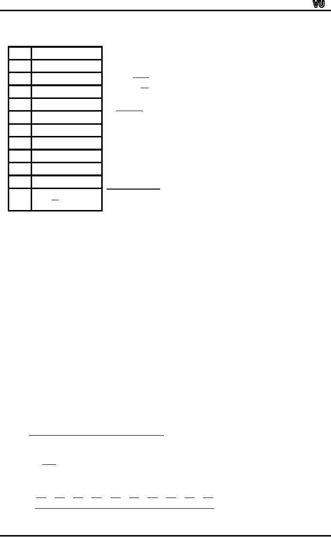
MTH001
Elementary Mathematics
where
n is the no. of
terms)
We
have:
X
1/X
30
1/30
= 0.0333
n
H.M.
=
35
1/35
= 0.0286
1
∑
40
1/40
= 0.0250
X
10
40
1/40
= 0.0250
=
45
1/45
= 0.0222
0.2488
40
1/40
= 0.0250
=
40.2 mph
50
1/50
= 0.0200
55
1/55
= 0.0182
Hence
it is clear that the
55
1/55
= 0.0182
harmonic
mean gives the
30
1/30
= 0.0333
totally
correct result.
1
=
0.2488
∑
X
The
key question is, "When
should we compute the
harmonic mean of a data
set?"
The
answer to this question will
be easy to understand if we consider
the following rules:
RULES
1.
When
values are given as x per y
where x is constant and y is
variable, the
Harmonic
Mean
is the appropriate average to
use.
2.
When
values are given as x per y
where y is constant and x is
variable, the
Arithmetic
Mean is the appropriate
average to use.
3.
When
relative changes in some
variable quantity are to be
averaged, the
geometric
mean
is the appropriate average to
use.
We
have already discussed the
geometric and the harmonic
means.
Let
us now try to understand
Rule No. 1 with the
help of an example:
EXAMPLE:
If
10 students have obtained
the following marks (in a
test) out of 20:
13,
11, 9, 9, 6,
5,
19, 17, 12, 9
Then
the average marks (by
the formula of the
arithmetic mean) are:
13
+
11
+
9
+
9
+
6
+
5
+
19
+
17
+
12
+
9
10
110
=
=
11
10
This
is equivalent to
13
11 9
9
6
5
19 17 12 9
+
+
+
+
+
+
+
+
+
20
20 20 20 20 20 20 20 20
20
10
Page
186

MTH001
Elementary Mathematics
110
110
11
=
20
=
=
(i.e.
the average10arks
of�his
grou0
of
students are 11 out of
20).
10
t
20
2 p
m
In
the above example, the
point to be noted was that
all the marks were
expressible
as
x per y where the
denominator y was constant
i.e. equal to 20, and
hence, it was
appropriate
to compute the arithmetic
mean.
Let
us now consider a mathematical
relationship exists between
these
three
measures of central
tendency.
RELATION
BETWEEN ARITHMETIC,
GEOMETRIC
AND
HARMONIC MEANS:
Arithmetic
Mean > Geometric Mean
>Harmonic Mean
We
have considered the five
most well-known measures of
central tendency i.e.
arithmetic
mean,
median, mode, geometric mean
and harmonic mean.
It
is interesting to note that
there are some other
measures of central tendency as
well.
Two
of these are the mid
range, and the mid
quartile range.
Let
us consider these one by
one:
MID-RANGE:
If
there are n observations
with x0 and xm as their
smallest and largest
observations
respectively,
then their mid-range is
defined as
x0 +
xm
mid
-
range
=
2
It
is obvious that if we add
the smallest value with
the largest, and divide by
2, we will get a
value
which is more or less in the
middle of the
data-set.
MID-QUARTILE
RANGE:
If
x1, x2... xn are n observations
with Q1 and Q3 as their
first and
third
quartiles respectively, then
their mid-quartile range is
defined as
Q1 +
Q3
mid
-
quartile
range =
2
Similar
to the case of the
mid-range, if we take the
arithmetic mean of the upper
and lower
quartiles,
we will obtain a value that
is somewhere in the middle of
the data-set.
The
mid-quartile range is also
known as the
mid-hinge.
Let
us now revise briefly the
core concept of central
tendency:
Masses
of data are usually
expressed in the form of
frequency tables
so
that it becomes easy to
comprehend the data.
Usually,
a statistician would like to go a
step ahead and to compute a
number that will
represent
the data in some definite
way.
Any
such single number that
represents a whole set of
data is called `Average'.
Technically
speaking, there are many
kinds of averages (i.e.
there are several ways
to
compute
them). These quantities that
represent the data-set are
called "measures of
central
tendency".
Page
187
Table of Contents:
- Recommended Books:Set of Integers, SYMBOLIC REPRESENTATION
- Truth Tables for:DE MORGAN’S LAWS, TAUTOLOGY
- APPLYING LAWS OF LOGIC:TRANSLATING ENGLISH SENTENCES TO SYMBOLS
- BICONDITIONAL:LOGICAL EQUIVALENCE INVOLVING BICONDITIONAL
- BICONDITIONAL:ARGUMENT, VALID AND INVALID ARGUMENT
- BICONDITIONAL:TABULAR FORM, SUBSET, EQUAL SETS
- BICONDITIONAL:UNION, VENN DIAGRAM FOR UNION
- ORDERED PAIR:BINARY RELATION, BINARY RELATION
- REFLEXIVE RELATION:SYMMETRIC RELATION, TRANSITIVE RELATION
- REFLEXIVE RELATION:IRREFLEXIVE RELATION, ANTISYMMETRIC RELATION
- RELATIONS AND FUNCTIONS:FUNCTIONS AND NONFUNCTIONS
- INJECTIVE FUNCTION or ONE-TO-ONE FUNCTION:FUNCTION NOT ONTO
- SEQUENCE:ARITHMETIC SEQUENCE, GEOMETRIC SEQUENCE:
- SERIES:SUMMATION NOTATION, COMPUTING SUMMATIONS:
- Applications of Basic Mathematics Part 1:BASIC ARITHMETIC OPERATIONS
- Applications of Basic Mathematics Part 4:PERCENTAGE CHANGE
- Applications of Basic Mathematics Part 5:DECREASE IN RATE
- Applications of Basic Mathematics:NOTATIONS, ACCUMULATED VALUE
- Matrix and its dimension Types of matrix:TYPICAL APPLICATIONS
- MATRICES:Matrix Representation, ADDITION AND SUBTRACTION OF MATRICES
- RATIO AND PROPORTION MERCHANDISING:Punch recipe, PROPORTION
- WHAT IS STATISTICS?:CHARACTERISTICS OF THE SCIENCE OF STATISTICS
- WHAT IS STATISTICS?:COMPONENT BAR CHAR, MULTIPLE BAR CHART
- WHAT IS STATISTICS?:DESIRABLE PROPERTIES OF THE MODE, THE ARITHMETIC MEAN
- Median in Case of a Frequency Distribution of a Continuous Variable
- GEOMETRIC MEAN:HARMONIC MEAN, MID-QUARTILE RANGE
- GEOMETRIC MEAN:Number of Pupils, QUARTILE DEVIATION:
- GEOMETRIC MEAN:MEAN DEVIATION FOR GROUPED DATA
- COUNTING RULES:RULE OF PERMUTATION, RULE OF COMBINATION
- Definitions of Probability:MUTUALLY EXCLUSIVE EVENTS, Venn Diagram
- THE RELATIVE FREQUENCY DEFINITION OF PROBABILITY:ADDITION LAW
- THE RELATIVE FREQUENCY DEFINITION OF PROBABILITY:INDEPENDENT EVENTS