 |
Median in Case of a Frequency Distribution of a Continuous Variable |
| << WHAT IS STATISTICS?:DESIRABLE PROPERTIES OF THE MODE, THE ARITHMETIC MEAN |
| GEOMETRIC MEAN:HARMONIC MEAN, MID-QUARTILE RANGE >> |
MTH001
Elementary Mathematics
LECTURE #
25:
� Median in
case of a frequency distribution of a
continuous variable
� Median in
case of an open-ended frequency
distribution
� Empirical
relation between the mean,
median and the
mode
�
Quantiles
(quartiles, deciles &
percentiles)
�
Graphic
location of quantiles.
Median
in Case of a Frequency Distribution of a
Continuous Variable:
In
case of a frequency distribution,
the median is given by the
formula
h
⎛n ⎞
~
X
=
l
+
⎜ - c⎟
f
⎝2 ⎠
Where
l
=lower class boundary of the
median class (i.e. that
class for which the
cumulative
frequency
is just in excess of
n/2).
h=class
interval size of the median
class
f
=frequency of the median
class
n=Σf
(the total number of
observations)
c
=cumulative frequency of the
class preceding the median
class
Note:
This
formula is based on the
assumption that the
observations in each class
are evenly
distributed
between the two class
limits.
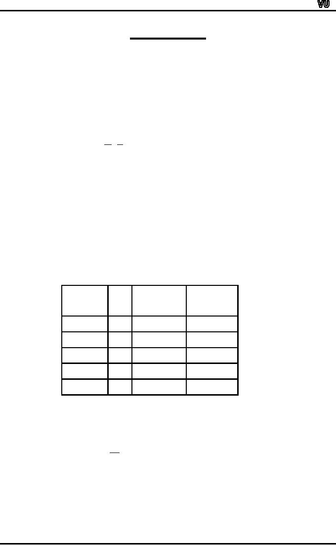
Example:
Going
back to the example of the
EPA mileage ratings, we
have
No.
Mileage
Class
Cumulative
of
Rating
Boundaries
Frequency
Cars
30.0
32.9
2
29.95
32.95
2
33.0
35.9
4
32.95
35.95
6
36.0
38.9
14
35.95
38.95
20
39.0
41.9
8
38.95
41.95
28
42.0
44.9
2
41.95
44.95
30
In
this example, n = 30 and n/2
= 15.
Thus
the third class is the
median class. The median
lies somewhere between 35.95
and
38.95.
Applying the above formula,
we obtain
3
~
(15
-
6)
X
=
35.95
+
14
=
35.95
+
1.93
=
37.88
~
37.9
-
Interpretation:
Page
171
MTH001
Elementary Mathematics
This
result implies that half of
the cars have mileage
less than or up to 37.88
miles per
gallon
whereas the other half of
the cars has mileage
greater than 37.88 miles
per gallon.
As
discussed earlier, the
median is preferable to the
arithmetic mean when there
are a few
very
high or low figures in a
series. It is also exceedingly
valuable when one encounters
a
frequency
distribution having open-ended
class intervals.
The
concept of open-ended frequency
distribution can be understood
with the help of
the
following
example.
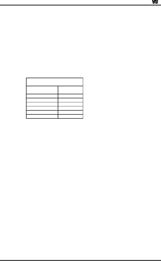
WAGES
OF WORKERS
Example:
IN
A FACTORY
Monthly
Income
No.
of
(in
Rupees)
Workers
Less
than 2000/-
100
2000/-
to 2999/-
300
3000/-
to 3999/-
500
4000/-
to 4999/-
250
5000/-
and above
50
Total
1200
In
this example, both the
first class and the
last class are open-ended
classes. This is so
because
of the fact that we do not
have exact figures to begin
the first class or to end
the
last
class. The advantage of
computing the median in the
case of an open-ended
frequency
distribution
is that, except in the
unlikely event of the median
falling within an
open-ended
group
occurring in the beginning of
our frequency distribution,
there is no need to
estimate
the
upper or lower boundary.
This is so because of the
fact that, if the median is
falling in an
intermediate
class, then, obviously, the
first class is not being
involved in its
computation.The
next concept that we will
discuss is the empirical
relation between the
mean,
median and the mode.
This is a concept which is
not based on a rigid
mathematical
formula;
rather, it is based on observation. In
fact, the word `empirical'
implies `based on
observation'.
This
concept relates to the
relative positions of the
mean, median and
the
mode
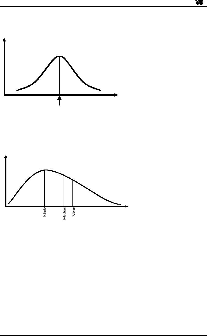
in case of a hump-shaped distribution. In
a single-peaked frequency distribution,
the
values
of the mean, median and
mode coincide if the
frequency distribution is
absolutely
symmetrical.
Page
172
MTH001
Elementary Mathematics
THE
SYMMETRIC CURVE
f
X
Mean
= Median = Mode
But
in the case of a skewed
distribution, the mean,
median and mode do not
all lie on the
same
point. They are pulled
apart from each other,
and the empirical relation
explains the
way
in which this happens.
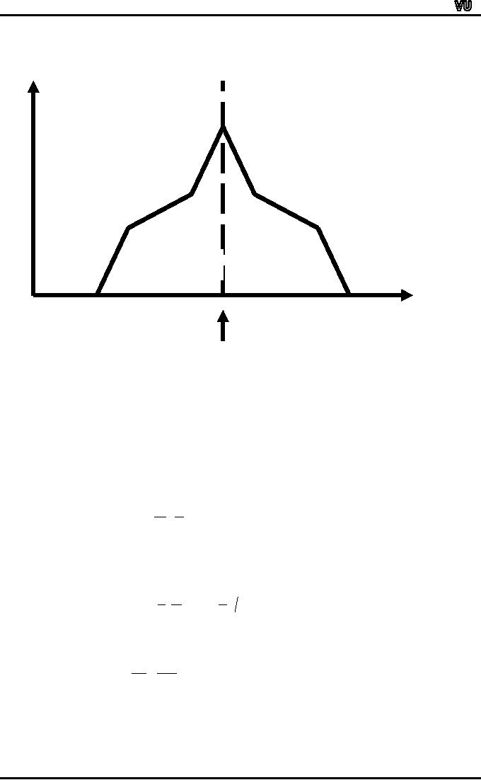
Experience tells us that in a
unimodal curve of
moderate
skewness,
the median is usually
sandwiched between the mean
and the mode.
The
second point is that, in the
case of many real-life
data-sets, it has
been
observed
that the distance between
the mode and the
median is approximately double
of
thf
distance
between the median and
the mean, as shown
below:
e
X
This
diagrammatic picture is equivalent to
the following algebraic
expression:
Median
- Mode
2
(Mean - Median) ----
(1)
The
above-mentioned point can
also be expressed in the
following way:
Mean
Mode =
3
(Mean Median)
----
(2)
Equation
(1) as well as equation (2)
yields the approximate
relation given below:
EMPIRICAL
RELATION BETWEEN
THE
MEAN, MEDIAN AND THE MODE
:
Mode
= 3 Median 2 Mean
An
exactly similar situation
holds in case of a moderately
negatively skewed
distribution.
An
important point to note is
that this empirical relation
does not hold in case of
a
J-shaped
or an extremely skewed
distribution.
Let
us now extend the concept of
partitioning of the frequency
distribution by
taking
up the concept of quantiles
(i.e. quartiles, deciles and
percentiles).
Page
173
MTH001
Elementary Mathematics
We
have already seen that
the median divides the
area under the frequency
polygon into
two
equal halves:
f
50%
50%
X
Median
A
further split to produce
quarters, tenths or hundredths of
the total area under
the
frequency
polygon is equally possible,
and may be extremely useful
for analysis. (We
are
often
interested in the highest
10% of some group of values
or the middle 50%
another.)
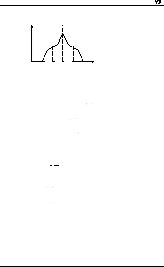
QUARTILES
The
quartiles, together with the
median, achieve the division
of the total area into
four equal
parts.
The
first, second and third
quartiles are given by the
formulae:
First
quartile:
⎛n
⎞
h
Q1 =
l
+
⎜
- c⎟
f
⎝4
⎠
Second
quartile (i.e.
median):
h⎛2n ⎞
h
Q
=l+
⎜ -c⎟=l+
(n
2-c)
2
f⎝4 ⎠
f
Third
quartile:
h
⎛
3n
⎞
= l +
-
c⎟
⎜
Q
3
f ⎝ 4
⎠
It
is clear from the formula of
the second quartile that
the second quartile is the
same as the
median.
Page
174
MTH001
Elementary Mathematics
f
25%
25% 25% 25%
X
~
Q1 Q2 =
X
Q3
DECILES
& PERCENTILES
The
deciles and the percentiles
given the division of the
total area into 10 and
100 equal
parts
respectively.
The
formula for the first
decile is
h⎛ n ⎞
D1 =
l
+ ⎜
- c⎟
The
formulae for the subsequent
deciles afe⎝10
⎠
r
h
⎛
2n
⎞
D2 =
l
+ ⎜
- c⎟
f
⎝
10
⎠
h
⎛
3n
⎞
D3 =
l
+
-
c⎟
⎜
f
⎝
10
⎠
and
so on.
It
is easily seen that the
5th decile is the same
quantity as the
median.
The
formula for the first
percentile is
h⎛ n ⎞
P
=l+ ⎜
-c⎟
1
f
⎝100
⎠
The
formulae for the subsequent
percentiles are
h
⎛
2n
⎞
P2 =
l
+
⎜
-
c⎟
f
⎝100
⎠
⎛
3n
⎞
h
P3 =
l
+
-
c⎟
⎜
f
⎝
100
⎠
and
so on.
Again,
it is easily seen that the
50th percentile is the same
as the median, the
25th
percentile
is the same as the 1st
quartile, the 75th
percentile is the same as
the 3rd quartile,
the
40th percentile is the same
as the 4th decile, and so
on.
All
these measures i.e. the
median, quartiles, deciles
and percentiles are
collectively
called quantiles. The
question is, "What is the
significance of this concept
of
partitioning?
Why
is it that we
wish to divide our frequency
distribution into two, four,
ten or
hundred
parts?"
Page
175
MTH001
Elementary Mathematics
The
answer to the above
questions is: In certain
situations, we may be interested
in
describing
the relative
quantitative
location of a particular measurement
within a data set.
Quantiles
provide us with an easy way
of achieving this. Out of
these various quantiles,
one
of
the most frequently used is
percentile ranking.
Let
us understand this point
with the help of an
example.
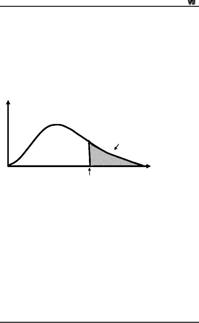
EXAMPLE:
If
oil company `A' reports
that its yearly sales
are at the 90th percentile
of all companies in
the
industry, the implication is
that 90% of all oil
companies have yearly sales
less
than
company
A's, and only 10%
have yearly sales exceeding
company A's:
This
is demonstrated in the following
figure:
Rel
ativ
e
Fre
que
ncy
0.10
0.90
Yearly
Company
A's sales
(90th
percentile)
It
is evident from the above
example that the concept of
percentile ranking is quite a
useful
concept,
but it should be kept in
mind that percentile
rankings are of practical
value only for
large
data sets.
It
is evident from the above
example that the concept of
percentile ranking is quite a
useful
concept,
but it should be kept in
mind that percentile
rankings are of practical
value only for
large
data sets.
The
next concept that we will
discuss is the graphic
location of quantiles.
Let
us go back to the example of
the EPA mileage ratings of 30
cars
that
was
discussed
in an earlier lecture. The
statement of the example
was:
EXAMPLE:
Suppose
that the Environmental
Protection Agency of a developed
country performs
extensive
tests on all new car
models in order to determine
their mileage rating.
Suppose
that the following 30
measurements are obtained by
conducting such tests on
a
particular
new car model.
Page
176
MTH001
Elementary Mathematics
ILEAGE
RATINGS ON 30 CARS (MILES PER
GALLON)
42.1
44.9
37.5
32.9
40.0
40.2
35.6
35.9
38.8
38.6
38.4
40.5
39.0
37.0
36.7
37.1
34.8
33.9
38.1
39.8
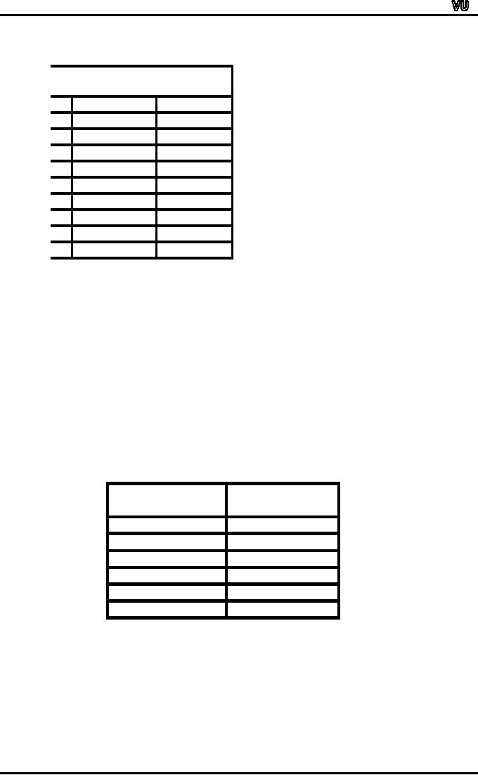
When
the above data was
converted to a frequency distribution, we
obtained:
Class
Limit
Frequency
30.0
32.9
2
33.0
35.9
4
36.0
38.9
14
39.0
41.9
8
42.0
44.9
2
30
Also,
we considered the graphical
representation of this
distribution.
The
cumulative frequency polygon of
this distribution came out
to be as shown in the
following
figure:
Page
177
MTH001
Elementary Mathematics
Cumulative
Frequency Polygon or
OGIVE
35
30
25
20
15
10
5
0
5
5
5
5
5
5
.9
.9
.9
.9
.9
.9
44
41
8
5
2
9
3
3
3
2
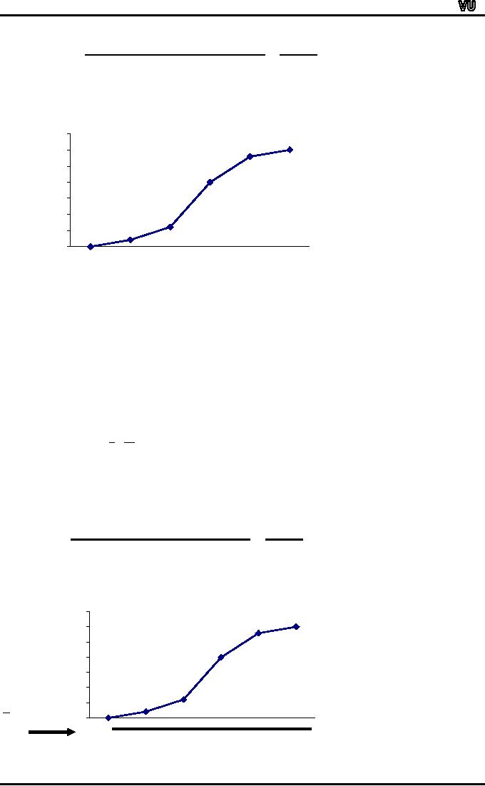
This
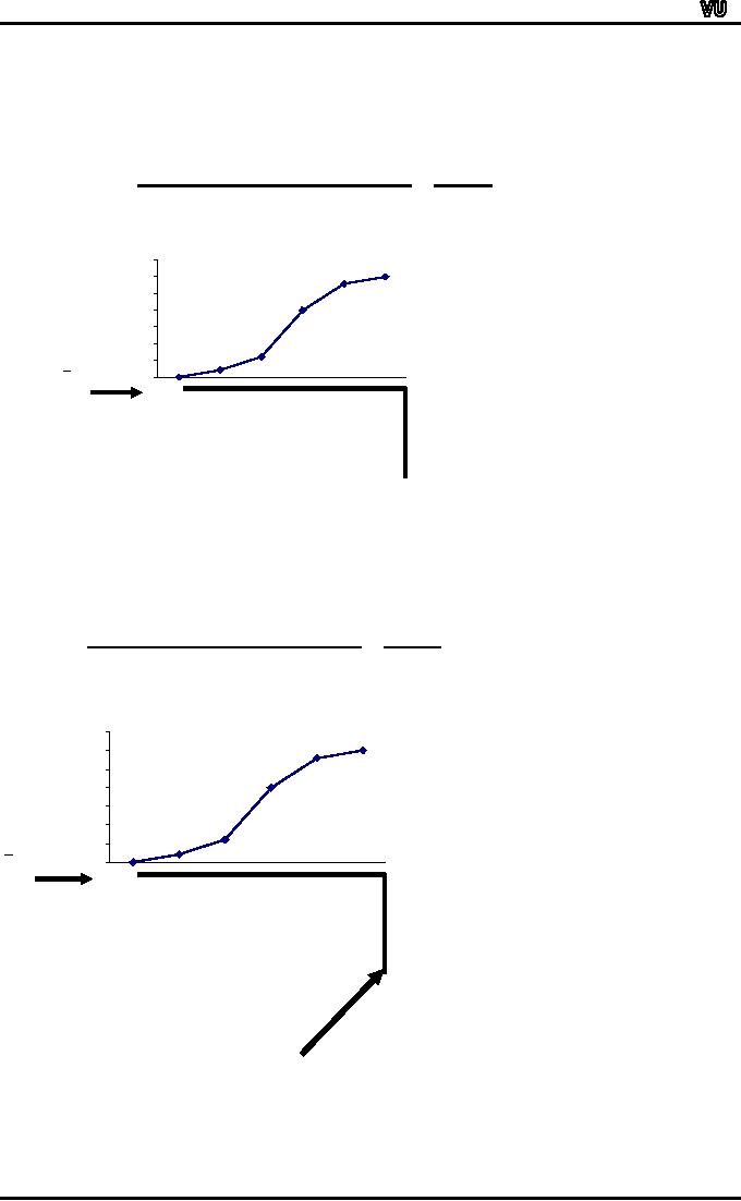
ogive enables us to find the
median and any other
quantile that we may be
interested in
very
conveniently. And this process is
known as the graphic
location of quantiles.
Let
us begin with the graphical
location of the
median:
Because
of the fact that the
median is that value before
which half of the
data
lies,
the first step is to divide
the total number of
observations n by 2.
In
this example:
n
30
=
=
15
2 2
The
next step is to locate this
number 15 on the y-axis of
the cumulative frequency
polygon.
Cumulative
Frequency Polygon or
OGIVE
35
30
25
20
15
10
5
n
0
2
95
95
95
95
95
95
4.
1.
8.
5.
9.
2.
4
4
3
3
2
3
Page
178
MTH001
Elementary Mathematics
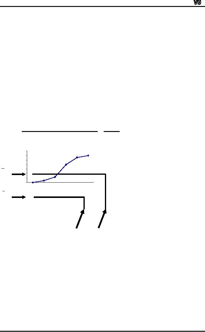
Lastly,
we drop a vertical line from
the cumulative frequency
polygon down to the
x-axis.
Cumulative
Frequency Polygon or
OGIVE
35
30
25
20
15
10
5
n
0
2
5
5
5
5
5
5
.9
.9
.9
.9
.9
.9
44
41
38
35
32
29
Now,
if we read the x-value where
our perpendicular touches
the x-axis, students, we
find
that
this value is approximately
the same as what we obtained
from our formula.
Cumulative
Frequency Polygon or
OGIVE
35
30
25
20
15
10
5
n
0
2
5
5
5
5
5
5
.9
.9
.9
.9
.9
.9
44
41
38
35
32
29
~
X
=
37.9
It
is evident from the above
example that the cumulative
frequency polygon is a very
useful
device
to find the value of the
median very quickly.In a
similar way, we can locate
the
Page
179
MTH001
Elementary Mathematics
quartiles,
deciles and percentiles.To
obtain the first quartile,
the horizontal line will be
drawn
against
the value n/4, and
for the third quartile,
the horizontal line will be
drawn against the
value
3n/4.
Cumulative
Frequency Polygon or
OGIVE
35
30
25
20
3n
15
4
10
5
0
5
5
5
5
95
5
.9
.9
.9
.9
.9
n
.
44
41
38
35
32
29
4
Q3
Q1
For
the deciles, the horizontal
lines will be against the
values n/10, 2n/10, 3n/10,
and so on.
And
for the percentiles, the
horizontal lines will be
against the values n/100,
2n/100, 3n/100,
and
so on.
The
graphic location of the
quartiles as well as of a few
deciles and
percentiles
for
the data-set of the EPA
mileage ratings may be taken
up as an exercise:
This
brings us to the end of our
discussion regarding quantiles
which are sometimes
also
known
as fractiles --- this
terminology because of the
fact that they divide
the frequency
distribution
into various parts or
fractions.
Page
180
Table of Contents:
- Recommended Books:Set of Integers, SYMBOLIC REPRESENTATION
- Truth Tables for:DE MORGAN’S LAWS, TAUTOLOGY
- APPLYING LAWS OF LOGIC:TRANSLATING ENGLISH SENTENCES TO SYMBOLS
- BICONDITIONAL:LOGICAL EQUIVALENCE INVOLVING BICONDITIONAL
- BICONDITIONAL:ARGUMENT, VALID AND INVALID ARGUMENT
- BICONDITIONAL:TABULAR FORM, SUBSET, EQUAL SETS
- BICONDITIONAL:UNION, VENN DIAGRAM FOR UNION
- ORDERED PAIR:BINARY RELATION, BINARY RELATION
- REFLEXIVE RELATION:SYMMETRIC RELATION, TRANSITIVE RELATION
- REFLEXIVE RELATION:IRREFLEXIVE RELATION, ANTISYMMETRIC RELATION
- RELATIONS AND FUNCTIONS:FUNCTIONS AND NONFUNCTIONS
- INJECTIVE FUNCTION or ONE-TO-ONE FUNCTION:FUNCTION NOT ONTO
- SEQUENCE:ARITHMETIC SEQUENCE, GEOMETRIC SEQUENCE:
- SERIES:SUMMATION NOTATION, COMPUTING SUMMATIONS:
- Applications of Basic Mathematics Part 1:BASIC ARITHMETIC OPERATIONS
- Applications of Basic Mathematics Part 4:PERCENTAGE CHANGE
- Applications of Basic Mathematics Part 5:DECREASE IN RATE
- Applications of Basic Mathematics:NOTATIONS, ACCUMULATED VALUE
- Matrix and its dimension Types of matrix:TYPICAL APPLICATIONS
- MATRICES:Matrix Representation, ADDITION AND SUBTRACTION OF MATRICES
- RATIO AND PROPORTION MERCHANDISING:Punch recipe, PROPORTION
- WHAT IS STATISTICS?:CHARACTERISTICS OF THE SCIENCE OF STATISTICS
- WHAT IS STATISTICS?:COMPONENT BAR CHAR, MULTIPLE BAR CHART
- WHAT IS STATISTICS?:DESIRABLE PROPERTIES OF THE MODE, THE ARITHMETIC MEAN
- Median in Case of a Frequency Distribution of a Continuous Variable
- GEOMETRIC MEAN:HARMONIC MEAN, MID-QUARTILE RANGE
- GEOMETRIC MEAN:Number of Pupils, QUARTILE DEVIATION:
- GEOMETRIC MEAN:MEAN DEVIATION FOR GROUPED DATA
- COUNTING RULES:RULE OF PERMUTATION, RULE OF COMBINATION
- Definitions of Probability:MUTUALLY EXCLUSIVE EVENTS, Venn Diagram
- THE RELATIVE FREQUENCY DEFINITION OF PROBABILITY:ADDITION LAW
- THE RELATIVE FREQUENCY DEFINITION OF PROBABILITY:INDEPENDENT EVENTS