 |
MTH001
Elementary Mathematics
Lecture #
24:
In
today's lecture, we will
continue with the concept of
the mode, and
will
discuss
the non-modal situation as
well as the bi-modal
situation.
First of
all, let us revise the
discussion carried out at
the end of the last
lecture.
You
will recall that we picked
up the example of the EPA
mileage ratings, and
computed
the mode of this
distribution by applying the
following formula:
Mode:
fm-f1
^
X=1+
xh
(fm-f1)
+(fm-f2)
Where
l
=
lower class boundary of the
modal class,
fm
=
frequency of the modal
class,
f1
=
frequency of the class
preceding the
modal
class,
f2
=
frequency of the class
following modal
class,
and
h
=
length of class interval of
the modal class
Hence,
we obtained:
14
-
4
^
=
35.95+
�3
X
(14- 4)
+ (14- 8)
10
=
35.95+
�3
10+ 6
=
35.95+1.875
=
37.825
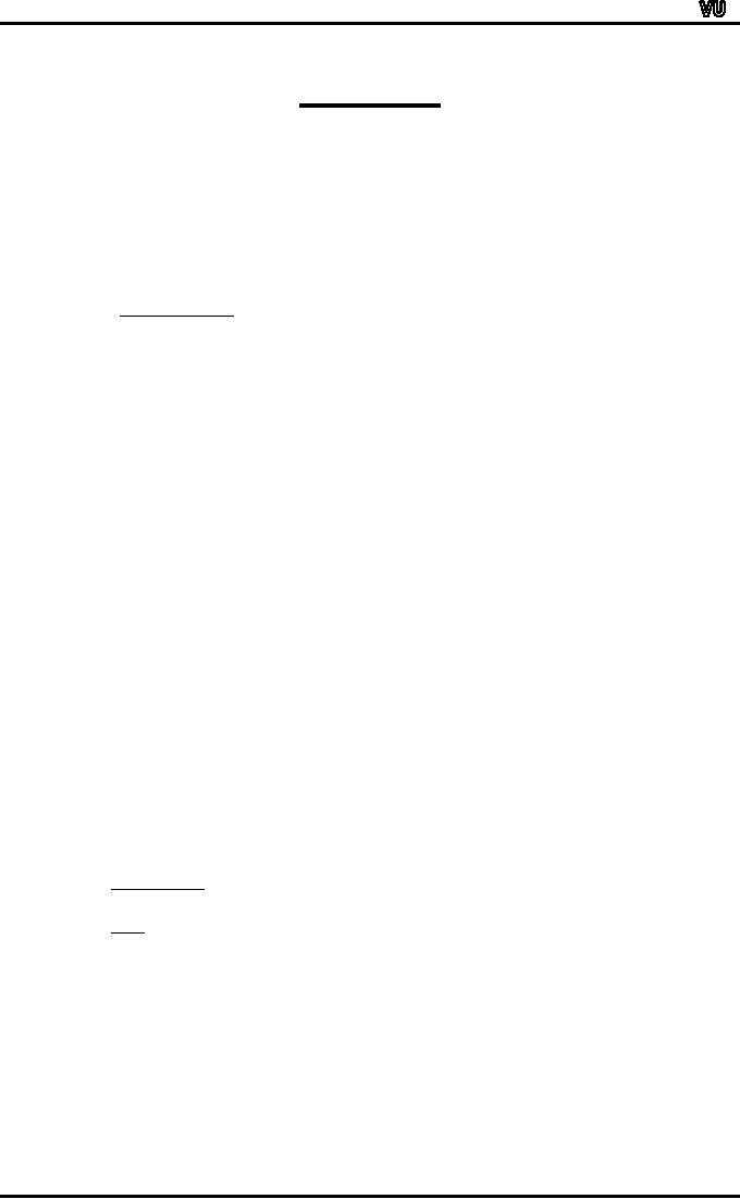
Subsequently,
we considered the location of
the mode with reference
to
the
graphical
picture
of our frequency
distribution.
Page
158
MTH001
Elementary Mathematics
Y
16
14
12
10
8
6
4
2
0
X
Miles
per gallon
^
X
=
37.825
In
general, it was noted that,
for most of the frequency
distributions, the mode
lies
somewhere
in the middle of our
frequency distribution, and
hence is eligible to be called
a
measure
of central tendency.
The
mode has some very
desirable properties.
DESIRABLE
PROPERTIES OF THE
MODE:
�
The
mode is easily understood
and easily ascertained in
case of a discrete
frequency
distribution.
�
It is
not affected by a few very
high or low values.
The
question arises, "When
should we use the
mode?"
The
answer to this question is
that the mode is a valuable
concept in certain
situations
such as the one described
below:
Suppose
the manager of a men's
clothing store is asked
about the average size
of
hats
sold. He will probably think
not of the arithmetic or
geometric mean size, or
indeed the
median
size. Instead, he will in
all likelihood quote that
particular size which is
sold most
often.
This
average is of far more use
to him as a businessman than
the arithmetic mean,
geometric
mean or the median. The
modal size of all clothing
is the size which
the
businessman
must stock in the greatest
quantity and variety in
comparison with other
sizes.
Indeed,
in most inventory (stock
level) problems, one needs
the mode more often
than any
other
measure of central tendency. It
should be noted that in some
situations there may
be
no
mode in a simple series
where no value occurs more
than once.
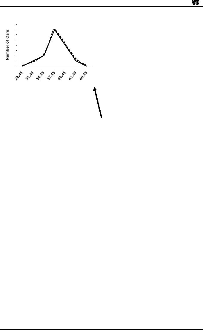
On
the other hand, sometimes a
frequency distribution contains
two modes in
which
case it is called a bi-modal
distribution as shown
below:
Page
159
MTH001
Elementary Mathematics
THE
BI-MODAL FREQUENCY
DISTRIBUTION
f
X
0
The
next measure of central
tendency to be discussed is the
arithmetic mean.
THE
ARITHMETIC MEAN
The
arithmetic mean is the
statistician's term for what
the layman knows as the
average. It
can
be thought of as that value of
the variable series which is
numerically
MOST
representative
of the whole series.
Certainly, this is the most
widely used average
in
statistics.
Easiest In addition, it is probably
the to calculate.
Its
formal definition is:
ARITHMETIC
MEAN:
The
arithmetic mean or simply
the mean is a value obtained
by dividing the sum of all
the
observations
by their number.
Arithmetic
Mean:
Sum
of all the
observations
X
=
Number
of the observations
n
∑
X
i
X
r of=obseirv=a1ions
in the sample that has
been the
n
Where
n represents the
numbe
t
ith
observation
in the sample (i = 1, 2, 3, ..., n),
and represents the mean of
the sample.
For
simplicity, the above
formula can be written
as
∑
X
X =
n
In
other words, it is not
necessary to insert the
subscript `i'.)
Page
160
MTH001
Elementary Mathematics
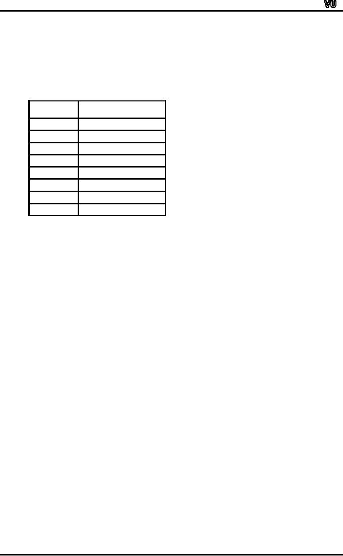
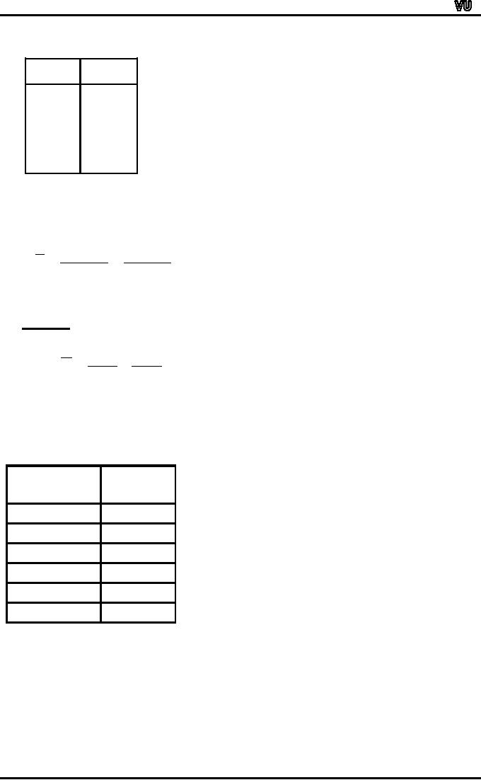
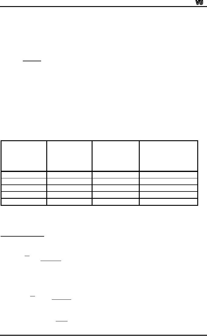
EXAMPLE:
Information
regarding the receipts of a
news agent for seven
days of a particular week
are
given
below
Day
Receipt
of News Agent
Monday
�
9.90
Tuesday
�
7.75
Wednesday
�
19.50
Thursday
�
32.75
Friday
�
63.75
Saturday
�
75.50
Sunday
�
50.70
Week
Total
�
259.85
Mean
sales per day in this
week:
=
� 259.85/7 = � 37.12
(To
the nearest penny).
Interpretation:
The
mean, � 37.12, represents
the amount (in pounds
sterling) that would have
been
obtained
on each day if the same
amount were to be obtained on
each day. The
above
example
pertained to the computation of
the arithmetic mean in case
of ungrouped data
i.e.
raw
data.
Let
us now consider the case of
data that has been
grouped into a
frequency
distribution.
When data pertaining to a
continuous variable has been
grouped into a
frequency
distribution, the frequency
distribution is used to calculate
the approximate
values
of
descriptive measures --- as
the identity of the
observations is lost.
To
calculate the approximate
value of the mean, the
observations in each class
are
assumed
to be identical with the
class midpoint Xi.
The
mid-point of every class is
known as its
class-mark.
In
other words, the midpoint of
a class `marks' that
class.As was just mentioned,
the
observations
in each class are assumed to
be identical with the
midpoint i.e. the
class-mark.
(This
is based on the assumption
that the observations in the
group are evenly
scattered
between
the two extremes of the
class interval).
As
was just mentioned,
the
observations in each class
are assumed to be
identical
with
the midpoint i.e. the
class-mark.(This
is based on the assumption
that the observations
in
the group are evenly
scattered between the two
extremes of the class
interval).
Page
161
MTH001
Elementary Mathematics
FREQUENCY
DISTRIBUTION
Mid
Point Frequency
X
f
X1
f1
X2
f2
X3
f3
:
:
:
:
:
:
Xk
fk
In
case of a frequency distribution,
the arithmetic mean is
defined as:
ARITHMETIC
MEAN
k
k
∑fX
∑fX
i
i
i
i
X=
=
i
=1
i
=1
k
n
∑
fi
i
=1
For
simplicity, the above
formula can be written
as
∑
fX
=
∑ fX
X=
∑f
n
(The
subscript `i' can be
dropped.)
Let
us understand this point
with the help of an
example:
Going
back to the example of EPA
mileage ratings that we
dealt with when discussing
the
formation
of a frequency distribution. The
frequency distribution that we
obtained was:
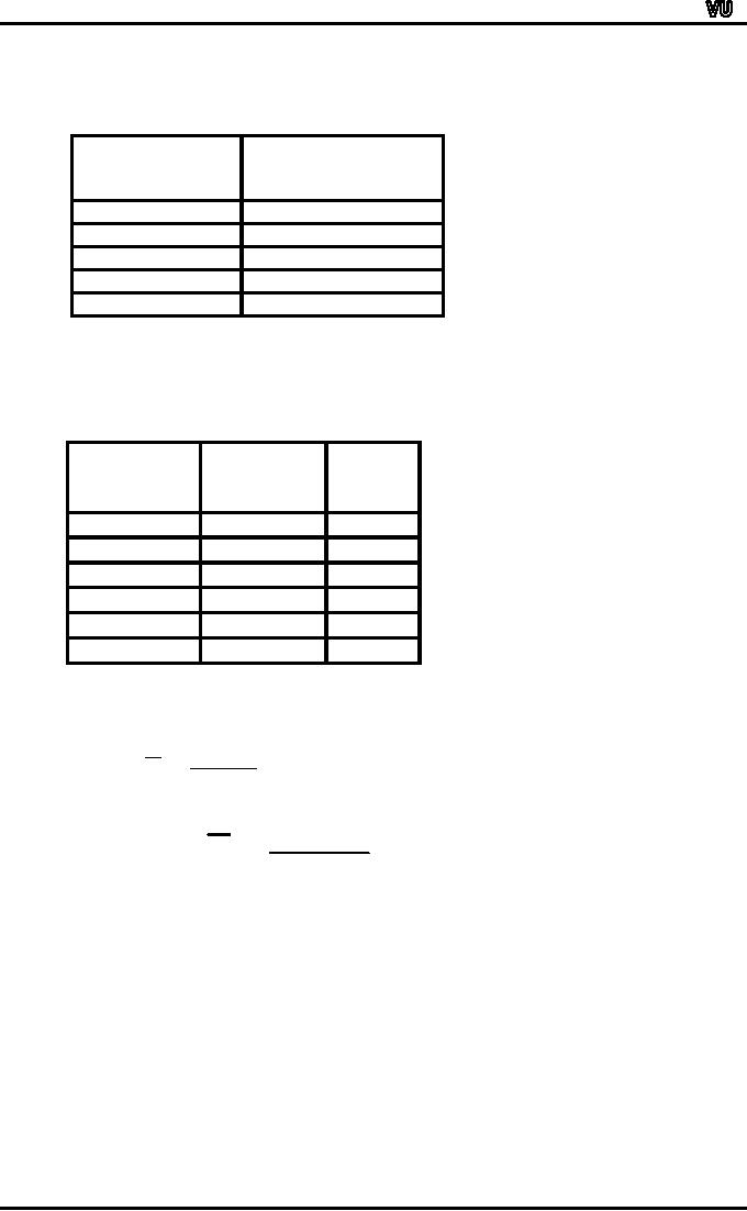
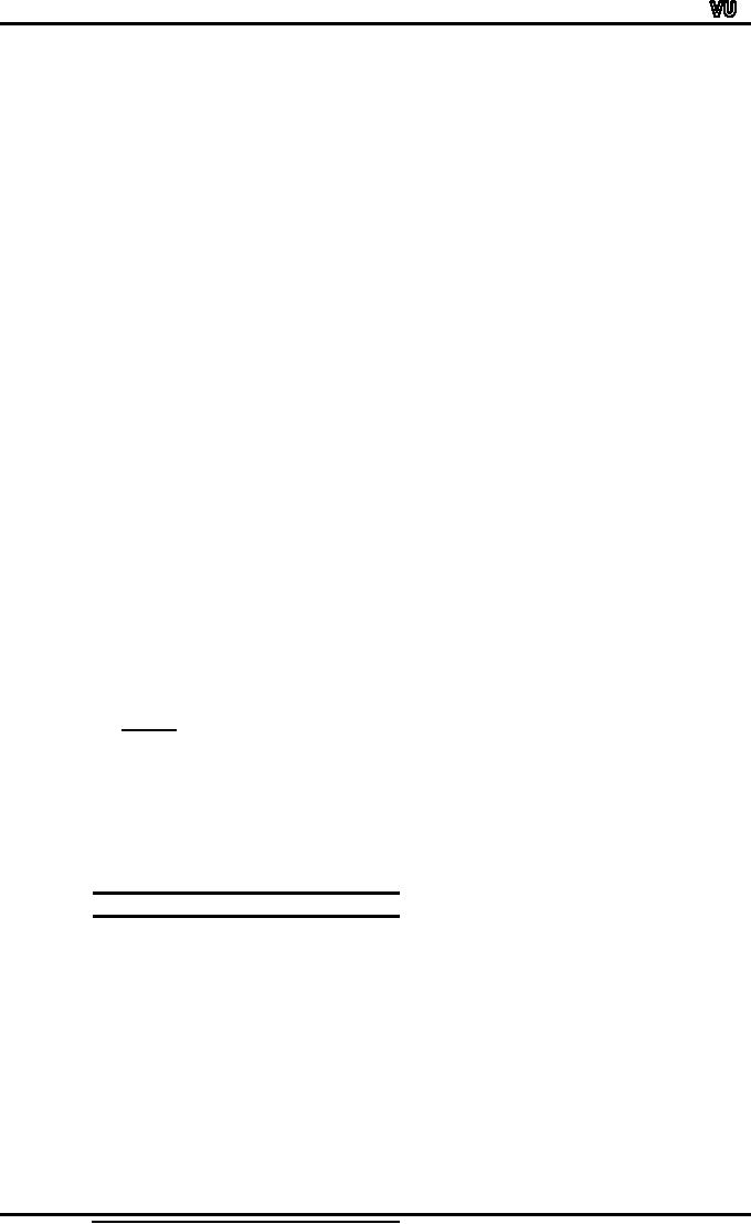
EPA
MILEAGE RATINGS OF 30 CARS OF A
CERTAIN MODEL
Class
Frequency
(Mileage
Rating) (No. of Cars)
30.0
32.9
2
33.0
35.9
4
36.0
38.9
14
39.0
41.9
8
42.0
44.9
2
Total
30
The
first step is to compute the
mid-point of every
class.
(You
will recall that the
concept of the mid-point has
already been discussed in an
earlier
lecture.)
CLASS-MARK
(MID-POINT):
The
mid-point of each class is
obtained by adding the sum
of the two limits of
the
class
and dividing by 2.
Page
162
MTH001
Elementary Mathematics
Hence,
in this example, our
mid-points are computed in
this manner:
30.0
plus 32.9 divided by 2 is
equal to 31.45,
33.0
plus 35.9 divided by 2 is
equal to 34.45,
And
so on.
Class
Class-mark
(Mileage
Rating)
(Midpoint)
X
30.0
32.9
31.45
33.0
35.9
34.45
36.0
38.9
37.45
39.0
41.9
40.45
42.0
44.9
43.45
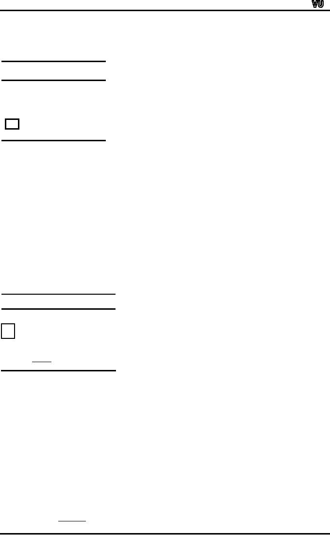
In
order to compute the
arithmetic mean, we first
need to construct the column
of fX, as
shown
below:
Class-mark
Frequency
fX
(Midpoint)
f
X
31.45
2
62.9
34.45
4
137.8
37.45
14
524.3
40.45
8
323.6
43.45
2
86.9
30
1135.5
Applying
the formula
∑
fX
X =
,
∑
f
We
obtain
1135
.5
X =
=
37
.85
30
INTERPRETATION:
The
average mileage rating of
the 30 cars tested by the
Environmental Protection Agency
is
37.85
on the average, these
cars run 37.85 miles
per gallon. An important
concept to be
discussed
at this point is the concept
of grouping error.
GROUPING
ERROR:
"Grouping
error" refers to the error
that is introduced by the
assumption that all
the
values
falling in a class are equal
to the mid-point of the
class interval. In reality, it is
highly
improbable
to have a class for which
all the values lying in
that class are equal to
the mid-
point
of that class. This is why
the mean that we calculate
from a frequency distribution
does
not
give exactly the same
answer as what we would get
by computing the mean of our
raw
data.
As
indicated earlier, a frequency
distribution is used to calculate
the approximate values
of
various
descriptive measures.(The word
`approximate' is being used
because of the
Page
163
MTH001
Elementary Mathematics
grouping
error that was just
discussed.) This grouping
error arises in the
computation of
many
descriptive measures such as
the geometric mean, harmonic
mean, mean deviation
and
standard deviation. But,
experience has shown that in
the calculation of the
arithmetic
mean,
this error is usually small
and never serious. Only a
slight difference occurs
between
the
true answer that we would
get from the raw
data, and the answer
that we get from
the
data
that has been grouped in
the form of a frequency
distribution.
In
this example, if we calculate
the arithmetic mean directly
from the 30 EPA
mileage
ratings,
we obtain:
Arithmetic
mean computed from raw
data of the EPA mileage
ratings:
363+301+.....
339+398
+ .
.
.
.
X=
30
1134
.7
=
=
37
.82
30
The
difference between the true
value of i.e. 37.82
and the value obtained
from the
frequency
distribution i.e. 37.85 is
indeed very slight. The
arithmetic mean is
predominantly
used
as a measure of central
tendency.
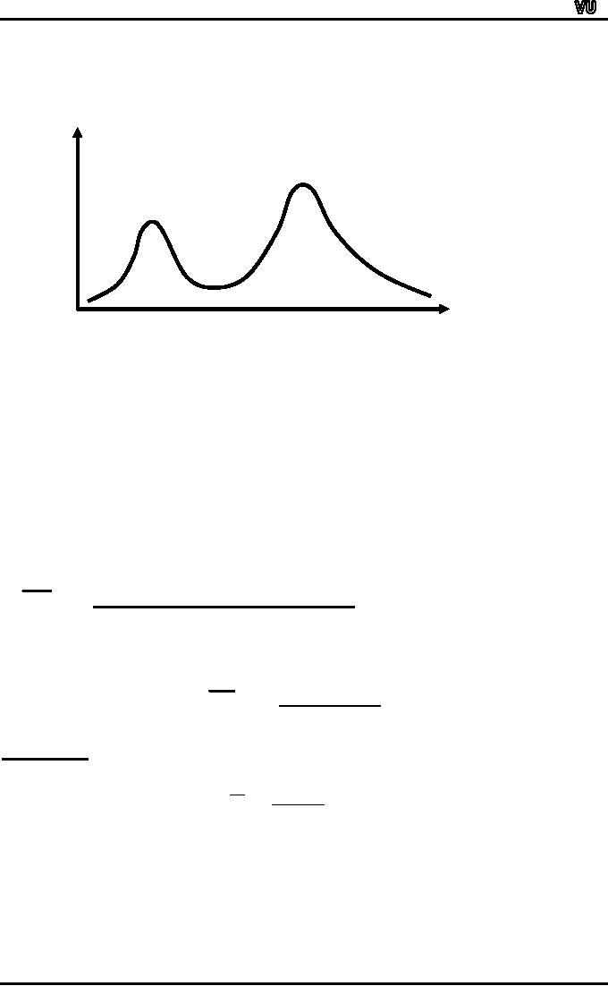
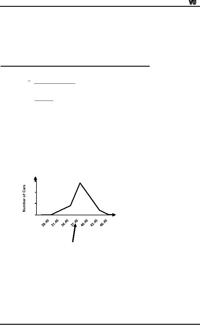
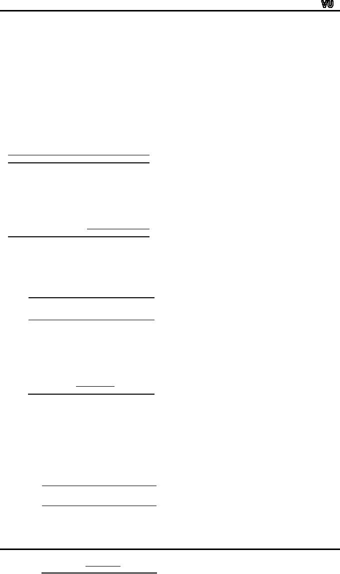
The
question is, "Why is it that
the arithmetic mean is known
as a measure of central
tendency?"
The
answer to this question is
that we have just obtained
i.e. 37.85 falls more or
less in the
centre
of our frequency
distribution.
Y
15
10
5
0
X
M
ile s pe r gallon
Mean
= 37.85
As
indicated earlier, the
arithmetic mean is predominantly
used as a measure of
central
tendency.
It
has many desirable
properties:
DESIRABLE
PROPERTIES OF THE ARITHMETIC
MEAN
�
Best
understood average in
statistics.
�
Relatively
easy to calculate
�
Takes
into account every value in
the series.
But
there is one limitation to
the use of the arithmetic
mean:
As
we are aware, every value in
a data-set is included in the
calculation of the
mean,
whether
the value be high or low.
Where there are a few
very high or very low
values in the
Page
164
MTH001
Elementary Mathematics
series,
their effect can be to
drag
the
arithmetic mean towards
them. this may make
the
mean
unrepresentative.
Example:
Example
of the Case Where the
Arithmetic Mean Is Not a
Proper Representative of
the
Data:
Suppose
one walks down the
main street of a large city
centre and counts the
number of
floors
in each building.
Suppose,
the following answers are
obtained:
5,
4, 3, 4, 5, 4, 3, 4, 5,
20,
5, 6, 32, 8, 27
The
mean number of floors is 9
even though 12 out of 15 of
the buildings have 6 floors
or
less.
The
three skyscraper blocks are
having a disproportionate effect on
the arithmetic mean.
(Some
other average in this case
would be more
representative.)
The
concept that we just
considered was the concept
of the simple arithmetic
mean.
Let
us now discuss the concept
of the weighted arithmetic
mean.
Consider
the following
example:
EXAMPLE:
Suppose
that in a particular high
school, there are:-
100
freshmen
80
sophomores
70
juniors
50
seniors
And
suppose that on a given day,
15% of freshmen, 5% of sophomores,
10% of juniors, 2%
of
seniors are absent.
The
problem is that: What
percentage of students is absent
for the school as a
whole
on
that particular day?
Now
a student is likely to attempt to
find the answer by adding
the percentages and
dividing
by
4 i.e.
15+ 5 +10+
2
32
=
=8
4
4
But
the fact of the matter is
that the above calculation
gives a wrong answer.In
order to
figure
out why this is a wrong
calculation, consider the
following:As we have already
noted,
15%
of the freshmen are absent
on this particular day.
Since, in all, there are
100 freshmen
in
the school, hence the
total number of freshmen who
are absent is also
15.
But
as far as the sophomores are
concerned, the total number
of them in the
school
is 80, and if 5% of them are
absent on this particular
day, this means that
the total
number
of sophomores who are absent
is only 4.
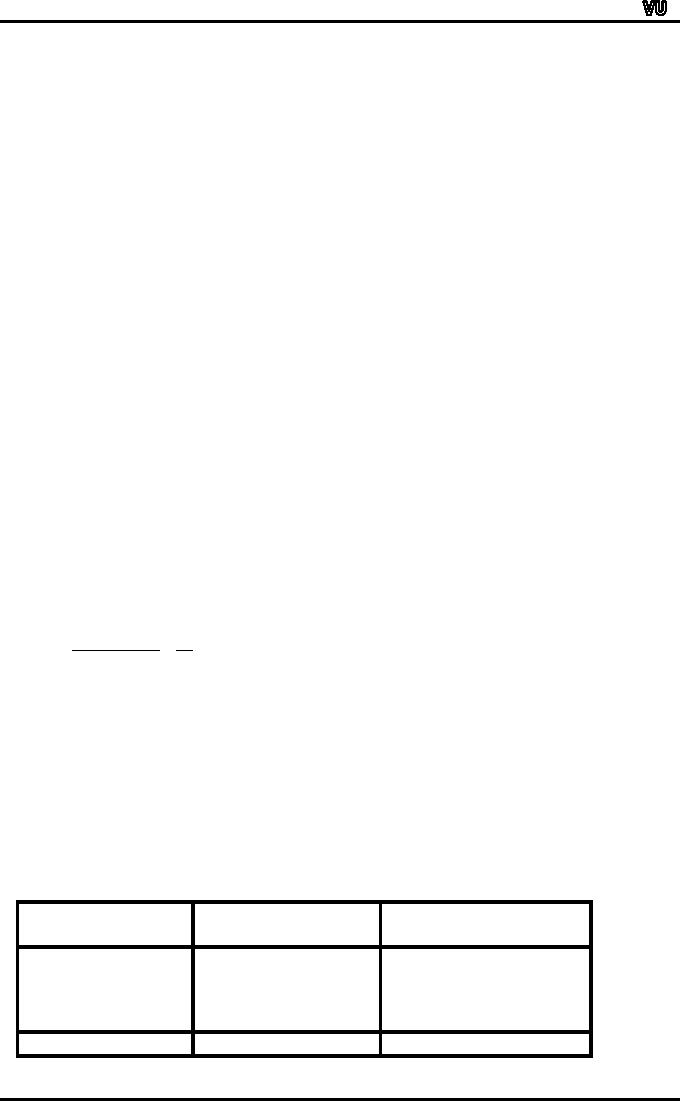
Proceeding
in this manner, we obtain
the following table.
Number
of Students in the
Number
of Students who are
Category
of Student
school
absent
Freshman
100
15
Sophomore
80
4
Junior
70
7
Senior
50
1
TOTAL
300
27
Page
165
MTH001
Elementary Mathematics
Dividing
the total number of students
who are absent by the
total number of
students
enrolled
in the school, and
multiplying by 100, we
obtain:
27
�
100
= 9
300
Thus
its very clear that
previous result was not
correct.
This
situation leads us to a very
important observation, i.e.
here our figures pertaining
to
absenteeism
in various categories of students
cannot be regarded as having
equal
weightage.
When
we have such a situation,
the concept of "weighing"
applies i.e. every data
value in
the
data set is assigned a
certain weight according to a
suitable criterion. In this
way, we will
have
a weighted series of data
instead of an un-weighted one. In
this example, the
number
of
students enrolled in each
category acts as the weight
for the number of
absences
pertaining
to that category i.e.
Number
of students
Percentage
of
enrolled
in the
WiXi
Students
who are
Category
of Student
school
(Weighted
Xi)
absent
(Weights)
Xi
Wi
100
�
15 =
1500
Freshman
15
100
80
�
5 =
400
Sophomore
5
80
70
�
10 =
700
Junior
10
70
50
�
2 =
100
Senior
2
50
ΣWi =
300
ΣWiXi
=
2700
Total
The
formula for the weighted
arithmetic mean is:
WEIGHTED
MEAN
∑WXi
Xw =
i
∑W
i
And,
in this example, the
weighted mean is equal
to:
∑
Wi Xi
=
Xw
∑
Wi
2700
=
300
=9
Page
166
MTH001
Elementary Mathematics
Thus
we note that, in this
example, the weighted mean
yields exactly the same as
the
answer
that we obtained
earlier.
As
obvious, the weighing
process leads us to a correct
answer under the
situation
where
we have data that cannot be
regarded as being such that
each value should be
given
equal
weightage.
An
important point to note here
is the criterion
for
assigning weights. Weights
can be
assigned
in a number of ways depending on
the situation and the
problem domain.
The
next measure of central
tendency that we will
discuss is the
median.
Let
us understand this concept
with the help of an
example.
Let
us return to the problem of
the `average' number of
floors in the buildings at
the centre of
a
city. We saw that the
arithmetic mean was
distorted towards the few
extremely high values
in
this series and became
unrepresentative.
We
could more appropriately and
easily employ the median as
the `average' in
these
circumstances.
MEDIAN:
The
median is the middle value
of the series when the
variable values are placed
in order of
magnitude.
MEDIAN:
The
median is defined as a value
which divides a set of data
into two halves,
one
half
comprising of observations greater
than and the other
half smaller than it.
More
precisely,
the median is a value at or
below which 50% of the
data lie.
The
median value can be
ascertained by inspection in many
series. For instance, in
this
very
example, the data that we
obtained was:
EXAMPLE-1:
The
average number of floors in
the buildings at the centre
of a city:
5,
4, 3, 4, 5, 4, 3, 4, 5, 20, 5, 6, 32, 8,
27
Arranging
these values in ascending
order, we obtain
3,
3, 4, 4, 4, 4, 5, 5, 5, 5, 6, 8, 20, 27,
32
Picking
up the middle value, we
obtain the median
equal
to 5.
Interpretation:
The
median number of floors is 5.
Out of those 15 buildings, 7
have upto 5 floors and 7
have
5
floors or more. We noticed
earlier that the arithmetic
mean was distorted toward
the few
extremely
high values in the series
and hence became
unrepresentative. The median = 5
is
much
more representative of this
series.
EXAMPLE-2:
Height
of buildings (number of
floors)
3
3
4
4
7
lower
4
5
5
5
= median height
5
5
6
8
7
higher
20
27
32
Page
167
MTH001
Elementary Mathematics
EXAMPLE-3:
Retail
price of motor-car
(�)
(several
makes and sizes)
415
480
4
above
525
608
719
= median price
1,090
2,059
4
above
4,000
6,000
A
slight complication arises
when there are even
numbers of observations in the
series, for
now
there are two middle
values.
The
expedient of taking the
arithmetic mean of the two
is adopted as explained
below:
EXAMPLE-4
Number
of passengers travelling on a
bus
at six Different times
during the day
4
9
14
=
median value
18
23
47
14
+
18
=
16 passengers
Median
=
2
Example
-5:
The
number of passengers traveling on a
bus at six different times
during a day are as
follows:
5,
14, 47, 34, 18,
23
Find
the median.
Solution:
Arranging
the values in ascending
order, we obtain
5,
14, 18, 23, 34,
47
As
before, a slight complication
has arisen because of the
fact that there are
even numbers
of
observations in the series
and, as such, there are
two middle values. As
before, we take
the
arithmetic mean of the two
middle values.
Hence
we obtain:
Median:
~
18 +
23
X=
=
20.5
passengers
2
Page
168
MTH001
Elementary Mathematics
A
very important point to be
noted here is that we must
arrange the data in
ascending order
before
searching for the two
middle values. All the
above examples pertained to
raw data.
Let
us now consider the case of
grouped data.
We
begin by discussing the case
of discrete data grouped
into a frequency
table.
As
stated earlier, a discrete
frequency distribution is no more
than a concise
representation
of
a simple series pertaining to a
discrete variable, so that
the same approach as the
one
discussed
just now would seem
relevant.
EXAMPLE
OF A DISCRETE FREQUENCY
DISTRIBUTION
Comprehensive
School:
Number
of pupils per
class
Number
of Classes
23
1
24
0
25
1
26
3
27
6
28
9
29
8
30
10
31
7
45
In
order to locate the middle
value, the best thing is to
first of all construct a
column of
cumulative
frequencies:
Comprehensive
School
Number
of
Number
of
Cumulative
pupils
per class
Classes
Frequency
X
f
cf
23
1
1
24
0
1
25
1
2
26
3
5
27
6
11
28
9
20
29
8
28
30
10
38
31
7
45
45
In
this school, there are 45
classes in all, so that we
require as the median that
class-size
below
which there are 22 classes
and above which also
there are 22 classes.
In
other words, we must find
the 23rd class in an ordered
list. We could simply count
down
noticing
that there is 1 class of 23
children, 2 classes with up to 25
children, 5 classes
with
up
to 26 children. Proceeding in this
manner, we find that 20
classes contain up to 28
children
whereas 28 classes contain up to 29
children. This means that
the 23rd class
---
the
one that we are looking
for --- is the one
which contains exactly 29
children.
Comprehensive
School:
Number
of
Number
of
Cumulative
pupils
per class
Classes
Frequency
X
f
cf
23
1
1
24
0
1
25
1
2
26
3
5
27
6
11
28
9
20
29
8
28
Virtual
University
of Pakistan 10
Page
30
38
169
31
7
45
45
MTH001
Elementary Mathematics
Median
number of pupils per
class:
~
X
=
29
This
means that 29 is the middle
size of the class. In other
words, 22 classes are such
which
contain
29 or less than 29 children,
and 22 classes are such
which contain 29 or more
than
29
children.
Page
170
Table of Contents:
- Recommended Books:Set of Integers, SYMBOLIC REPRESENTATION
- Truth Tables for:DE MORGAN’S LAWS, TAUTOLOGY
- APPLYING LAWS OF LOGIC:TRANSLATING ENGLISH SENTENCES TO SYMBOLS
- BICONDITIONAL:LOGICAL EQUIVALENCE INVOLVING BICONDITIONAL
- BICONDITIONAL:ARGUMENT, VALID AND INVALID ARGUMENT
- BICONDITIONAL:TABULAR FORM, SUBSET, EQUAL SETS
- BICONDITIONAL:UNION, VENN DIAGRAM FOR UNION
- ORDERED PAIR:BINARY RELATION, BINARY RELATION
- REFLEXIVE RELATION:SYMMETRIC RELATION, TRANSITIVE RELATION
- REFLEXIVE RELATION:IRREFLEXIVE RELATION, ANTISYMMETRIC RELATION
- RELATIONS AND FUNCTIONS:FUNCTIONS AND NONFUNCTIONS
- INJECTIVE FUNCTION or ONE-TO-ONE FUNCTION:FUNCTION NOT ONTO
- SEQUENCE:ARITHMETIC SEQUENCE, GEOMETRIC SEQUENCE:
- SERIES:SUMMATION NOTATION, COMPUTING SUMMATIONS:
- Applications of Basic Mathematics Part 1:BASIC ARITHMETIC OPERATIONS
- Applications of Basic Mathematics Part 4:PERCENTAGE CHANGE
- Applications of Basic Mathematics Part 5:DECREASE IN RATE
- Applications of Basic Mathematics:NOTATIONS, ACCUMULATED VALUE
- Matrix and its dimension Types of matrix:TYPICAL APPLICATIONS
- MATRICES:Matrix Representation, ADDITION AND SUBTRACTION OF MATRICES
- RATIO AND PROPORTION MERCHANDISING:Punch recipe, PROPORTION
- WHAT IS STATISTICS?:CHARACTERISTICS OF THE SCIENCE OF STATISTICS
- WHAT IS STATISTICS?:COMPONENT BAR CHAR, MULTIPLE BAR CHART
- WHAT IS STATISTICS?:DESIRABLE PROPERTIES OF THE MODE, THE ARITHMETIC MEAN
- Median in Case of a Frequency Distribution of a Continuous Variable
- GEOMETRIC MEAN:HARMONIC MEAN, MID-QUARTILE RANGE
- GEOMETRIC MEAN:Number of Pupils, QUARTILE DEVIATION:
- GEOMETRIC MEAN:MEAN DEVIATION FOR GROUPED DATA
- COUNTING RULES:RULE OF PERMUTATION, RULE OF COMBINATION
- Definitions of Probability:MUTUALLY EXCLUSIVE EVENTS, Venn Diagram
- THE RELATIVE FREQUENCY DEFINITION OF PROBABILITY:ADDITION LAW
- THE RELATIVE FREQUENCY DEFINITION OF PROBABILITY:INDEPENDENT EVENTS