Process of Dimensional Modeling: Four Step: Choose Business Process, Grain, Facts, Dimensions

<< Dimensional Modeling DM: ER modeling, The Paradox, ER vs. DM,

Issues of Dimensional Modeling: Additive vs Non-Additive facts, Classification of Aggregation Functions >>

Lecture-14

Process of Dimensional Modeling

The Process of Dimensional Modeling

Four Step Method from ER to DM

Choose the Business Process

Choose the Grain

Choose the Facts

Choose the Dimensions

A typical ER diagram covers the entire spectrum of the business, actually covers every possible

business process. However, in reality those multitudes of process do not co -exist in time and

space (tables). As a consequence, an ER diagram is overly complex, and is a demerit to itself.

This is precisely the point that differentiates a DM from an ER diagram, as a single ER diagram

can be divided into multiple DM diagrams. Thus a step-wise approach is followed to separate the

DMs from an ER diagram, and this consists of four steps.

Step -1: Separate the ER diagram into its discrete business processes and to model each business

process separately.

Step -2: Grain of a fact table = the meaning of one fact table row. Determines the maximum level

of detail of the warehouse.

Step -3: Select those many-to-many relationships in the ER model containing numeric and

additive non-key items and designate them as fact tables. Actually all business events to be

analyzed are gathered into fact tables.

Step -4: De-normalize all of the remaining tables into flat tables with single -part keys that connect

directly to the fact tables. These tables become the dimension tables. They are like reference

tables that define how to analyze the fact information. They are typically small and relatively

static.

Let's discuss each of the steps in detail, one by one.

S tep-1: Choose the Business Process

A business process is a major operational process in an organization.

Typically supported by a legacy system (database) or an OLTP.

§ Examples: Orders, Invoices, Inventory etc.

Business Processes are often termed as Data Marts and that is why many people criticize

DM as being data mart oriented.

The first step in DM is the business process selection. What do we mean by a process? A process

is a natural business activity in the organization supported by a legacy source data-collection

system (database or OLTP). Example business processes include purchasing, orders, shipments,

invoicing, inventory, and general ledger etc.

Many people consider business processes as Data marts i.e. in their view organizational or

depart mental function is referred as the business process. That is why such people criticize DM as

being a data mart oriented approach. However, in Kimball's view, it is a wrong approach, the

two must not be confused e.g. a single model is built to handle orders data rather than building

separate models for marketing and sales departments, which both access the orders data. By

focusing on business processes, rather than departments, consistent information can be delivered

economically throughout the organization . Building departmental data models may result in data

duplication, data inconsistencies, and data management issues. What is a possible solution? Yes,

publishing data once can not only reduce the consistency problems, but can also reduce ETL

development , data management and disk storage issues as well.

Step-1: Separating the Process

Figure-14.1: Step-1: Separating the Process

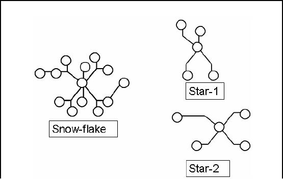
Fig-14.1 shows an interesting concept i.e. separating business processes to be modeled from a

complex set of processes. This translates to splitting a snow-flake schema into multiple star

schemas. Note that as the processes move into the star schema all the hierarchies collapse.

100

Step-2: Choosing the Grain

Grain is the fundamental, atomic level ofdata to be represented.

Grain is also termed as the unit of analyses.

Example grain statements

Typical grains

§ Individual Transactions

§ Daily aggregates (snapshots)

§ Monthly aggregates

Relationship between grain and expressiveness.

Grain vs. hardware trade-off.

Grain is the lowest level of detail or the atomic level of data stored in the warehouse. The lowest

level of data in the warehouse may not be the lowest level of data recorded in the business

system. It is also termed as the unit of analysis e.g. unit of weight is Kg etc.

Example grain statements: ( one fact row represents a...)

· Entry from a cash register receipt

· Boarding pass to get on a flight

· Daily snapshot of inventory level for a product in a warehouse

· Sensor reading per minute for a sensor

· Student enrolled in a course

Finer-grained fact tables:

· are more expressive

· have more rows

Trade -off between performance and expressiveness

· Rule of thumb: Err in favor of expressiveness

· Pre-computed aggregates can solve performance problems

In the absence of aggregates, there is a potential to waste millions of dollars on hardware

upgrades to solve performance problems that could have been otherwise addressed by

aggregates.

101

Step-2: Choosing the Grain

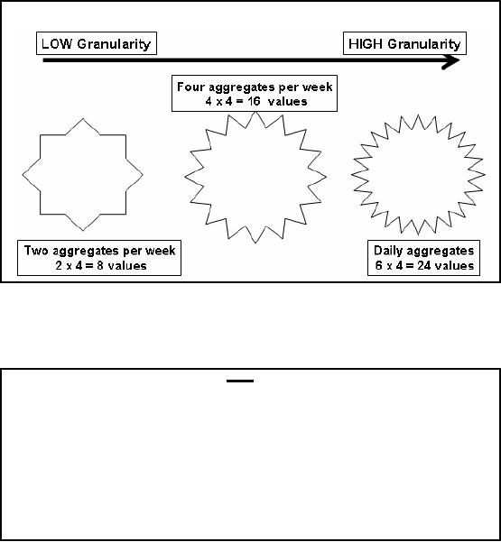
Figure-14.2: Step-2: Choosing the Grain

Note that you may come across definitions of grain as given in the notes and discussed in the

lectures, but you may also come across definitions that are different from those discussed. This

depends on the interpretation of the writer. We will follow the definition as per Fig-14.2.

The case FOR data aggregation

Works well for repetitive queries.

Follows the known thought process.

Justifiable if used for max number of queries.

Provides a "big picture" or macroscopic view.

Application dependent, usually inflexible to business changes (remember lack of

absoluteness of conventions).

There are both positives and negatives to data aggregation. These are a list of the reasons for the

utilization of summary or aggregate data . As you can see, they all really fall under the area of

"performance".

The negative side is that summary data does not allow a total solution with the flexibility and

capabilities that some businesses truly require as compared to other businesses.

102

The case AGAINST data aggregation

Aggregation is irreversible.

§ Can create monthly sales data from weekly sales data, but the reverse is not

possible.

Aggregation limits the questions that can be answered.

§ What, when, why, where , what-else, what-next

Aggregation can hide crucial facts.

§ The average of 100 & 100 is same as 150 & 50

Aggregation is one-way i.e. you can create aggregates, but can not dissolve aggregates to get the

original data from which the aggregates were created. For example 3+2+1 = 6 at the same time

2+4 also equals 6, so does 5+1 and if we consider reals, then infinetly many ways of adding

numbers to get the same result.

If you think about the "5 W's of journalism", these are the "6 W's of data analysis". Again it

highlights the types of questions that end users want to ask and can not be answered by summary

data.

By definition, a summarization will consider at least one of these points irrelevant. For example,

a summary across the company takes out the dimension of "WHERE" and a summary by quarters

takes out the element of "WHEN". The point to be noted is that although summary data has a

purpose, yet one can take any summary and ask a question that the system can not answer.

Aggregation hides crucial facts

Week -1 Week-2 Week -3 Week-4 Average

Zone-1

100

Just Looking at the averages i.e.

Zone-2

100

150

100

aggregates

Zone-3

100

150

100

Zone-4

200

100

Average

100

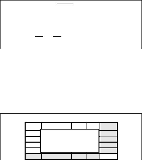
Table-14.1: Aggregation hides crucial facts

Consider the sales data of an item sold in a chain store in four zones, such that the sales data is

aggregated across the weeks also. For this simple example, for the sake of conserving space the

average sales across each zone and for each week is stored. Therefore, instead of storing 16

values only 8 values are stored i.e. a saving of 50% space.

Assume that a promotional scheme or advertisement campaign was run, and then the sales data

was recorded to analyze the effectiveness of the campaign. If we look at the averages (as shown

in the table) there is no change in sales i.e. neither across time nor across the geography

103

dimension. On the face of it, it was an in effective campaign. Now lets raise the curtain and look

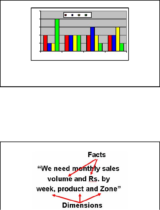
at the detailed sales records. The numbers are NOT constant! Drawing the graphs of the sales

records, shows a very different picture.

Aggregation hides crucial facts

250

200

150

100

Week-1

Week-2

Week-3

Week-4

Z1: Sale is

constant (need to work on it)

Z2: Sale went up, then fell (need of concern)

Z3: Sale is on the rise, why?

Z4: Sale dropped sharply, need to look deeply.

W2: Static sale

Figure-14.3: Aggregation hides crucial facts

Z1: Sale is constant through out the month (need to work on it)

Z2: Sale went up, then fell (need of concern) i.e. the campaign was effective, but after week it

fizzled down.

Z3: Sale is on the rise, why?

Z4: Sale dropped sharply, need to look deeply. It seems that the campaign had a negative effect

on the sales?

W2: Static sale across all zones, very unique indeed.

Step 3: Choose Facts

104

Numeric facts are identified by answering the question "what are we measuring?" Many- to-

many relationships in the ER model containing numeric and additive non -key items are selected

and designated as fact tables. In the example numeric additive figures volume (quantity ord ered)

and Rs. (Rupees cost amount) are the facts because the numeric values of the two are of keen

interest for the business user.

Step 3: Choose Facts

Choose the facts that will populate each fact table record.

Remember that best Facts are Numeric, Continuously Valued and Additive.

Example: Quantity Sold, Amount etc.

It should be remembered that facts are numeric, continuous, additive and non -key items that will

populate the fact table. Example facts for a point of sales terminal (POS) are sale s quantity, per

unit sales price, and the sales amount in rupees. All the candidate facts in a design must be true to

the grain described in previous slides. Facts that clearly belong to a different grain must be in a

separate fact table.

Step 4: Choose Dimensions

Choose the dimensions that apply to each fact in the fact table.

Typical dimensions: time, product, geography etc.

Identify the descriptive attributes that explain each dimension.

Determine hierarchies within each dimension.

Step-4: How to Identify a Dimension?

The single valued attributes during recording of a transaction are dimensions.

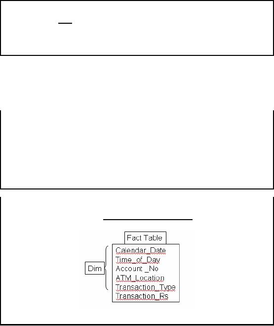
Time_of_day: Morning, Mid Morning, Lunch Break etc.

Transaction_Type: Withdrawal, Deposit, Check balance etc.

Table-14.2: Step-4: How to Identify a Dimension?

105

The dimension tables, usually represent textual attributes that are already known about things

such as the product, the geography, or the time. If the database designer is very clear about the

grain of the fact table, then choosing the appropriate dimensions for the fact table is usually easy.

What is so special about it, seems to be pretty intuitive, but is not.

The success in selecting the right dimensions for a given fact table is dependent on correctly

identifying any d scription that has a single value for an individual fact table record or

transaction. Note that the fact table record considered could be a single transaction or weekly

aggregate or monthly sums etc i.e. a grain is associated. Once this is correctly ident ified and

settled, then as many dimensions can be added to the fact able as required. For the ATM customer

transaction example, the following dimensions all have a single value during the recording of the

transaction, as none of the above dimensions change during a single transaction:

Calendar_Date

Time_of_Day

Account _No

ATM_Location

Transaction_Type (withdrawal, deposit, balance inquiry etc.)

Over here Time_of_Day refers to specific periods such as Morning, Mid Morning, Lunch Break,

Office_Off etc. Note that during an atomic transaction, the value of Time_of_Day does not

change (as a transaction takes less than a minute), hence it is a dimension. In the context of the

ATM example, the only numeric attribute is the Transaction_Rs, so it is a fact. Observe that we

use this convention in real life also, when people say we will visit you first time or second time of

the day etc.

Step-4: Can Dimensions be Multi-valued?

Are dimensions ALWYS single?

§ Not really

§ What are the problems? And how to handle them

How many maintenance operations are possible?

§ Few

§ Maybe more for old cars

Figure-14.4: Step-4: Can Dimensions be Multi-valued?

After convincing ourselves that dimensions are really single valued, perhaps we should consider

whether there are ever legitimate exceptions i.e. is it possible to have multi-valued dimension in a

fact table? If this is conceivable, what problems might arise?

Consider the following example from vehicle maintenance system used at a vehicle service

center. You are handed a data sheet for which the grain is the individual line item on the

customer's bill. The data source could be your periodic car maintenance visits to the company

106

workshop or individual replacement charges on a repair/change bill. These individual line items

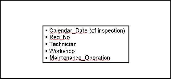
have a rich set of dimensions such as:

Calendar_Date (of inspection)

Reg_No (of vehicle)

Technician_ID

Workshop

Maintenance_Operation

The numeric additive facts in this design (which are the core of every fact table in a dimensional

design) would include Amount_Charged and perhaps others including Amount_Paid, depending

upon if the vehicle was insured etc.

On the face of it, this seems to be a very straightforward design, with obvious single values for all

the dimensions. But there is a surprise. In many situations, there may be multiple values for

services performed, such as oil change, air filter change, spark plug change etc. What do you do if

for a certain car there are three separate changes at the moment the service was performed? How

about really old and ill-kept cars that might have upto 5+ such changes? How do you encode the

Maintenance_Operation dimension if you wish to represent this information?

Step-4: Dimensions & Grain

Several grains are possible as per business requirement.

For some aggregations certain descriptions do not remain atomic.

Example: Time_of_Day may change several times during daily aggregate, but

not during a transaction

Choose the dimensions that are applicable within the selected grain.

Strangely, there is a relationship between the grain and the dimensions. When building a fact

table, the most important step is to declare the grain (aggregation level) of the fact table. The

grain declares the exact meaning of an individual fact record. Consider the case of transactions

for an ATM machine. The grain could be individual customer transaction, or number of

transaction per week or the amount drawn per month.

Calendar_Date

Time_of_Day

Account _No

ATM_Location

Transaction_Type (withdrawal, deposit, balance inquiry etc.)

Note that none of the above dimensions change during a single transaction. However, for weekly

transactions probably only Account _No and ATM_Location can be treated as a dimension.

Note that higher the level of aggregation of the fact table, the fewer will be the number of

dimensions you can attach to the fact records. The converse of this is surprising. The more

granular the data, the more dimensions make sense. Hence the lowest-level data in any

organization is the most dimensional.

107

Table of Contents: