OLAP Implementations: MOLAP, ROLAP, HOLAP, DOLAP

<< Online Analytical Processing OLAP: DWH and OLAP, OLTP

ROLAP: Relational Database, ROLAP cube, Issues >>

Lecture-11: Multidimensional OLAP (MOLAP)

OLAP Implementations

1. MOLAP: OLAP implemented with a multi-dimensional data structure.

2. ROLAP: OLAP implemented with a relational database.

3. HOLAP: OLAP implemented as a hybrid of MOLAP and ROLAP.

4. DOLAP: OLAP implemented for desktop decision support environments.

MOLAP physically builds "cubes" for direct access - usually in the proprietary file format of a

multi-dimensional database (MDD) or a user defined data structure. therefore ANSI SQL is not

supported.

ROLAP or a Relational OLAP provides access to information via a relational database using

ANSI standard SQL.

HOLAP provides a combination of relational database access and "cube" data structures within a

single framework. The goal is to get the best of both MOLAP and ROLAP: scalability (via

relational structures) and high performance (via pre -built cubes).

DOLAP allows download of "cube" structures to a desktop platform without the need for shared

relational or cube server. This model facilitates a mobile computing paradigm. DOLAP is

particularly useful for sales force automation types of applications by supporting extensive slide

and dice. A DOLAP implementation needs to be much more efficient in disk and memory

utilization than typical server implementations because computing power is often limited on a

laptop computer.

MOLAP Implementations

OLAP has historically been implemented using a multidimensional data structure or "cube".

Dimensions are key business factors for analysis:

§ Geographies (city, district, division, province,...)

§ Products (item, product category, product department,...)

§ Dates (day, week, month, quarter, year,...)

Very high performance achieved by O(1) time lookup into "cube" data structure to

retrieve pre_aggregated results.

Multi-dimensional databases (MDDs) typically use proprietary file formats to store pre -

summarized cube structures. There are dozens of vendors who provide MDD products. Essbase

from Hyperion and Powerplay from Cognos are some examples of market share leaders in this

space. Some RDBMS vendors have also begun packaging MDD capabilities into their product

offerings. Express from Oracle (acquired from IRI) and the MOLAP Store in Microsoft's OLAP

Server architecture (acquired from Panorama) are examples of products from RDBMS vendors.

MOLAP cubes are built around dimensions, as corresponding to each dimension is the index of

the multi-dimensional array data structure. Meaning, if there are four dimensions, then the data

will be stored in a four dimensional array i.e. with four indexes i, j, k and l. The other significance

of dimension from the business point of view are the key factors they correspond to, typically

dimensions are the features on which the WHERE clause is executed. Some examples of

dimension are geography, time, products etc. Note that typically dimensions have hierarchies, for

example geography dimension has the hierarchy of country, then province, then division, district,

city and zone as discussed in the last lecture.

The performance in a MOLAP cube comes from the O(1) look-up time for the array data

structure. Recall that to access an array, only the indexes are required i.e. there is no scanning of

the array (like a file data structure), there is no hashing it a constant access time operations,

similar to a random access memory (or RAM). The only time the time complexity goes beyond

O(1) is when the cube size is so large that it can not fit in the main memory, in such a case a page

or a block fault will occur.

MOLAP Implementations

No standard query language for querying MOLAP

- No SQL !

Vendors provide proprietary languages allowing business users to create queries that

involve pivots, drilling down, or rolling up.

- E.g. MDX of Microsoft

Languages generally involve extensive visual (click and drag) support.

Application Programming Interface (API)'s also provided for probing the cubes.

As it should be clear by now that, in a MOLAP environment there are no tables, there are no

traditional relational structures, hence ANSI SQL can not be used. As a matter of fact, there is no

standard query language for querying a MOLAP cube. The cube is sometimes probed by a

complex mapping mechanism that maps the user requirements into a set of indices, which are

then used to retrieve the aggregate from the corresponding matrix location. However, vendors

have come up with proprietary languages for non IT business users, the most popular being MDX

by Microsoft. These "languages" are graphical environments where the business users can click

on actions and perform drag-and-drop operations to provide input to retri eve data/information

from the cube. APIs are also available in the market for programming cube data retrieval by more

experienced programmers for running of complex quires. But none of these approaches use SQL.

Aggregations in MOLAP

Sales volume as a function of (i) product, (ii) time, and (iii) geography

A cube structure created to handle this.

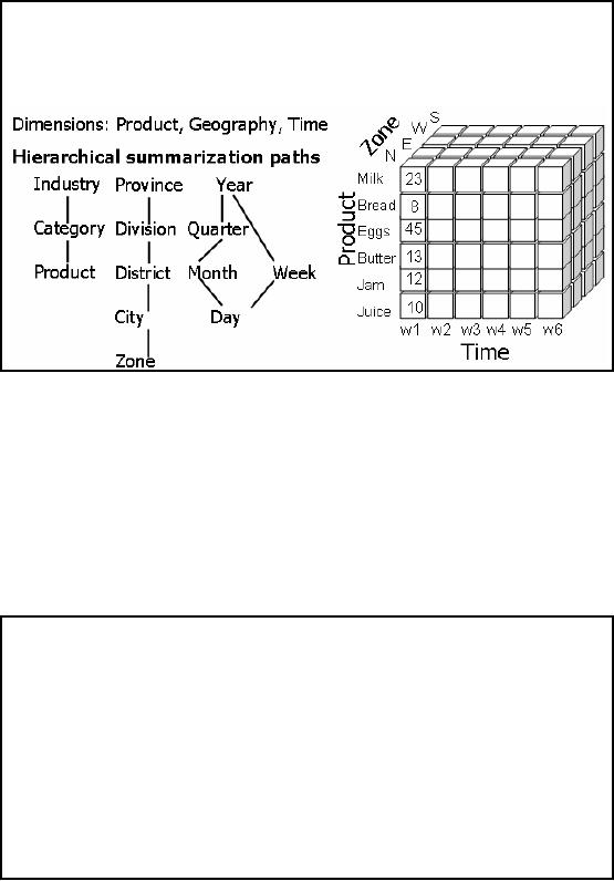
Figure-11.1: Filled cube

Figure11.1: Aggregation and a MOLAP cube

As already stated a number of times, in a Data Warehouse decision support environment we are

interested in the big picture, we want to look at the data from a macro level instead of the micro

level. For a macroscopic view aggregates are used. In this example we look at the sales volume

i.e. number of items sold as a function of product, time and geography. Note that all three of them

are dimensions. The proceed with the analysis, a cube structure will be first created such that each

dimension of the cube will correspond to each identified dimension, and within each dimension

will be the corresponding hierarchy. The example further shows how the dimensions are "rolled -

out" i.e. Province into divisions, then division into district, then district into city and finally cities

into zones. Note that weeks could be rolled into a year and at the same time months can be rolled

into quarters and quarters rolled into years. Based on these three dimensions a cube is created and

shown in figure -11.1.

Cube Operations

Rollup: summarize data

§ e.g., given sales data, summarize sales for last year by product category and

region

Drill down: get more details

§ e.g., given summarized sales as above, find breakup of sales by city within each

region, or within Sindh

Slice and dice: select and project

§ e.g.: Sales of soft -drinks in Karachi during last quarter

Pivot: change the view of data

The word cube is synonymously used with a MOLAP, therefore, when we talk of cube operations

we are never referring to SQL based querying, instead how we view the data stored in a cube.

There are four fundamental cubes operations which are (i) rollup (ii) drill down (iii) slice and dice

and (iv) pivoting. In the rollup operation the level of aggregation is increased i.e. data is presented

at a higher level of aggregation with less detail. For example while looking at the weekly sales

data, the decision maker decides to look at the monthly sales data, this is a rollup operation. On

the other hand, while looking at the weekly sales data, the decision makers wants to look at the

higher level of detail thus he/she drills down and looks at the daily sales data or was looking at

the division level of the sales data, and drills down into district level sales data by looking at the

sales in different cities corresponding to a district, among one of the many districts present in a

division. Slice and dice is a combination of looking at a subset of data based on more than one

dimension. As shown sin the slide, a combination of geography and time is used to look at part of

the cube across more than a singe dimension. Finally pivoting is changing the view of the data i.e.

replacing the dimension across the (say) x-axis. This will become clear when we look at specific

examples in the following slides.

Querying the Cube

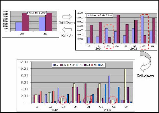
Figure-11.2: Different cube operations

Question: Juices are selling well or the sodas?

Looking at the highest level summary, with the lowest data granularity, shows that the sales of

Soda Drinks are higher for years 2001 and 2002.

Question: Which sodas are doing well?

Just clicking on the Sodas column shows the second histogram. It shows that the sales of 8-UP

cola are highest in both years i.e. 2001 and 2002.

Question: Is 8-UP a clear winner?

Flipping the dimensions i.e. instead of product on xaxis putting time on xaxis and further

drilling -down shows that there is a trend of increasing sales of 8-UP, BUT the sale is alarmingly

down during QTR3 in 2001 and QTR1 and QTR3 during 2002.

All of the above information was extracted by exploring 46 table entries and three levels of

aggregates. The total exploration time took less than 3 seconds.

Question: Why erratic sales of 8-UP?

This may probably require exploring other dimensions or their combinations.

Querying the Cube: Pivoting

Fig-11.3(a)

Fig-11.3(b)

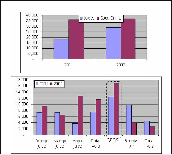
Figure-11.3: Pivot cube operations

This is a good exa mple of pivoting. In the first figure (11.3(a)), along x-axis we have the time

dimension, y-axis is the sales volumes, but volumes for the product are under two categories i.e.

juices and soda drinks. By the pivoting operation, the dimensions are interchanged, and we end

up with having the product along the x axis and the yearly sales figures (i.e. time dimension)

along the y-axis. The purpose of pivoting and other operations are not just to provide a set of

different operations, but to enable the decision maker to look at the data from different angles.

From fig-11.3(a) it seems that the sales of soda drinks are up consistently through year 2001 and

2002, but after pivoting and doing a drilldown operation, we see that the sales of apple juice was

higher than all soda drinks, except 8-UP, but the sale of 8-UP was so high both in years 2001 and

2002, that it shot up the overall sales of soda drinks. Thus all soda drinks are not the winners;

actually Pola -Kola has the weakest sales of all.

MOLAP Evaluation

Advantages of MOLAP:

Instant response (pre -calculated aggregates).

Impossible to ask question without an answer.

Value added functions (ranking, % change).

MOLAP implementations with pre-defined cubes as pre -aggregated data perform very well when

compared to relational databases, but often have difficulty scaling when the size of dimensions

becomes large. The breakpoint is typically around 64,000. Some implementations are also

limited to a file size for the cube representation that must be less than 2GB (this is less often an

issue than a few years ago).

Actually the cubes are less than 1% full.

MOLAP Evaluation

Drawbacks of MOLAP:

Long load time ( pre -calculating the cube may take days!).

Very sparse cube (wastage of space) for high cardinality (sometimes in small hundreds).

e.g. number of heaters sold in Jacobabad or Sibi.

A MOLAP is in no way a win -win situation, it has its won intrinsic pitfalls, which does not make

it an overall winner. The biggest drawback is the extremely long time taken to pre-calculate the

cubes, remember that in a MOLAP all possible aggregates are computed. The number of

aggregates suffers from something called as the "curse of dimensionality" i.e. as the number of

dimensions increases, the number of possible agg regates increases exponentially, this will be

further clarified in an upcoming slide. Because of long calculation times, cube creation is a batch

process and usually has the lowest priority and scheduled to be done late in the night. This

actually turns out to be a big mistake (as we will discuss subsequently) as it may so happen that

the cube generation may not actually take place, and the decision makers are presented with the

old and stale data, and they tend to lose faith in the OLAP paradigm. Although the number of

possible aggregates is very large, but NOT all the aggregates may have values, there can be and

will be quite a few aggregates which will have null values. For example, many of the items sold

in winter are not sold in summer and not even kept in the store (and vice-a-versa). Consequently,

there are no corresponding sales, and if the cube is generated that includes all the items, there will

be many null aggregates, resulting in a very sparse cube. This will result in requirement of large

amount of memory, most of which would be wasted. For these very reasons cube compression is

a hot area of research and development. We will not discuss it any further.

MOLAP Implementation Issues

Maintenance issue: Every data item received must be aggregated into every cube (assuming "to-

date" summaries are maintained). Lot of work.

Storage issue: As dimensions get less detailed (e.g., year vs. day) cubes get much smaller, but

storage consequences for building hundreds of cubes can be significant. Lot of space.

Scalability:

Often have difficulty scaling when the size of dimensions becomes large. The breakpoint is

typically around 64,000 cardinality of a dimension.

Maintenance Considerations: Every data item received into MDD must be aggregated into every

cube (assuming "to-date" summaries are maintained). Have to update the cubes every time a

change occurs (insert, delete, update), otherwise the user will run into synchronization problems.

Storage Considerations: Although cubes get much smaller (e.g., more dense) as dimensions get

less detailed (e.g., year vs. day), storage implications for building hundreds of cubes can be

significant. The reason being, as each possible combination of dimensions has to be pre -

calculated i.e. every combination of every a gregate, so soon faced with a combinatorial

explosion. Therefore, the number of entries in each dimension has to be of some reasonable

number. If you have entries above 100 in each dimension then things tend to blow up. When does

it actually blows up depends on the tool being used and how sparse matrices are stored. So you

might end up requiring more cube space then allocated or even available. Consider taking each

data element by week, and then 65 weeks times' geography is one cube. Now consider taking

each data element by month, this is a different cube i.e. by geography by 12 months, and then a

different cube by geography by year and so on. So the combinatorial explosion gets way out of

hand.

Scalability:

MOLAP implementations with pre-defined cubes as pre -aggregated data perform very well when

compared to relational databases, but often have difficulty scaling when the size of dimensions

becomes large. The breakpoint is typically around 64,000 cardinality of a dimension. Typically

beyond tens (sometimes small hundreds) of thousands of entries in a single dimension will break

the MOLAP model because the pre -computed cube model does not work well when the cubes are

very sparse in their population of individual cells. Some implementations are also limited to a file

size for the cube representation that must be less than 2GB (this is less often an issue than a few

years ago). You just can not build cubes big enough, or enough of them to have every thing pre -

computed. So you get into the problems of scale. As already discussed, it is difficult to scale

because of combinatorial explosion in the number and size of cubes when dimensions of

significant cardinality are required. There are two possible, but limited solutions addressing the

scalability problem i.e. Virtual cubes and partitioned cubes.

Partitioned Cubes

To overcome the space limitation of MOLAP, the cube is partitioned.

One logical cube of data can be spread across multiple physical cubes on separate (or

same) servers.

The divide&conquer cube partitioning approach helps alleviate the scalability limitations

of MOLAP implementation.

Ideal cube partitioning is completely invisible to end users.

Performance degradation does occur in case of a join across partitioned cubes.

When the cardinality of a dimension forces a cube to become larger than what can reasonably be

supported in a single cube, it is common practice to partition the cube into multiple "sub-cube"

instantiations. The sub-cubes are usually defined around logical partitions within the dimensional

hierarchies. For example, if there are a large number of entries at the most detailed level in a

product hierarchy, it may be advisable to create distinct cubes along product category boundaries

to divide-and-conquer. Another example would be to take a geographical dimension and partition

into cubes whereby each region has its own cube.

Advanced MOLAP implementations (e.g., Microsoft Analytic/OLAP Services) will automatically

distribute queries across partitioned cubes (potentially on distinct server platforms) for parallel

retrieval without exposing the end user to the underlying physical deployment of the partitioned

cubes.

Partitioned Cubes: How it looks Like?

Sales data cube partitioned at a major cotton pr oducts sale outlet

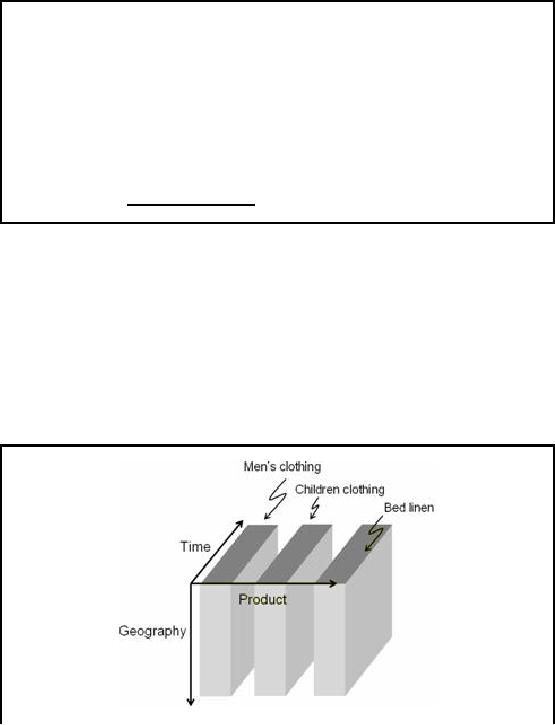
Figure-11.4: Partitioned Cube

There is unlikely to be a relationship between the sales of men's and children's clothing, thus the

sales cube is partitioned, as shown in figure-11.4. Usually when men buy, they buy for

themselves in most cases, except of course when they buying a gift for someone. When women

buy, they may also buy for the children, but not men. But then this may be incorrect for a certain

culture, hence is not a rule of thumb.

Bed linen is something very different, henc e the original single cube of all sales aggregates can be

partitioned along these two logical boundaries into three cubes which require less storage space

per cube. As MOLAP is intrinsically main memory resident, hence cube partitioning does not

results in notable speed-up, but does results in memory requirements, if for most queries one or

two cube partitions are required with infrequent joins across them.

Virtual Cubes

Used to query two dissimilar cubes by creating a third "virtual" cube by a join between two

cubes.

Logically similar to a relational view i.e. linking two (or more) cubes along common

dimension(s).

Biggest advantage is saving in space by eliminating storage of redundant information.

Example: Joining the store cube and the list price cube along the product dimension, to calculate

the sale price without redundant storage of the sale price data.

Advanced MOLAP implementations will often facilitate the creation of virtual cubes by

combining multiple cubes (at run-time) along common dimensions between cubes.

There is a run -time cost to "joining" across cubes at the time of query execution, but the savings

in storage can be quite large by eliminating redundancy in the underlying data representation.

Typically, the virtual cubes involve "joining" cubes along common dimensions whereby one cube

has a (smaller) subset of the dimensions from the other (bigger) cube.

Example: Usually the sale price of different items varies based on the geography and the time of

the year. Instead of storing this information using an additional dimension, the said price is

calculated at run-time, this may be slow, but can result in tremendous saving in space, as all the

items are not sold throughout the year.

Table of Contents: