AGGREGATE PLANNING:Aggregate Planning Relationships, Master Scheduling

<< AGGREGATE PLANNING:Demand and Capacity Options

INVENTORY MANAGEMENT:Objective of Inventory Control, Inventory Counting Systems >>

Production and Operations Management MGT613

Lesson 30

AGGREGATE PLANNING

Learning Objectives

In this lecture we will cover the basic aggregate planning strategies, Assumptions for Aggregate

Planning, different Aggregate Planning Relationships, Master Schedule and Master Scheduler. We will

study desegregating the aggregate plans for production control. This discussion would prepare us to

take a deeper look into Inventory Management and MRP/ERP. All this would allow us to become

effective operations manager to work for improving the operations as well as the systems of the

organizations we will work for.

Basic Strategies

Level capacity strategy: Maintaining a steady rate of regular-time output while meeting

variations in demand by a combination of options.

Chase demand strategy: Matching capacity to demand; the planned output for a period is set at

the expected demand for that period.

Chase Approach

Advantages

1. Investment in inventory is low

2. Labor utilization in high

Disadvantages

1. The cost of adjusting output rates and/or workforce levels

Level Approach

Advantages

1. Stable output rates and workforce

Disadvantages

1. Greater inventory costs

2. Increased overtime and idle time

3. Resource utilizations vary over time

Techniques for Aggregate Planning

Determine demand for each period

Determine capacities for each period

Identify policies that are pertinent

Determine units costs

Develop alternative plans and costs

Select the best plan that satisfies objectives. Otherwise return to step 5.

Assumptions for Aggregate Planning

1. The regular output capacity is the same for all periods.

2. Cost (Back Order, Inventory, Subcontracting etc) is a linear function composed of unit cost and

number of units. ( In reality cost is more of a step function)

3. Plans are feasible ( There is sufficient inventory exists to accommodate a plan, subcontractors

would provide quality products and outsourcers would be secure)

4. Assumptions for Aggregate Planning

5. All costs associated with a decision option can be represented by a lump sum or by unit costs

that are independent of the quantity involved.

6. Cost figures can be reasonably estimated and are constant over the planning horizon.

138

Production and Operations Management MGT613

7. Inventories are built up and draw down at a uniform rate and output occurs at a uniform rate

throughout each period. Backlogs are treated as if they exist for the entire period, even though

in reality they tend to build up towards the end of the period

Aggregate Planning Relationships

1. Number of workers in a period equals Number of Workers at the end of the previous period

PLUS Number of new Workers at the start of the current period - Number of laid off Workers at

the start of the current period

2. NOTE: SINCE the organization would not hire and layoff simultaneously, so at least one of the

last two terms will be "0".

3. Inventory at the end of a ( current) period equals Inventory at the end of the previous period

PLUS Production in the current period Amount used to satisfy the demand in the current

period

4. NOTE :The average Inventory for a period is equal to (Beginning Inventory Plus Ending

Inventory)/2

Average Inventory

Aggregate Planning Relationships

·Cost for a ( current) period equals Output Cost ( Regular +OT+ Subcontract) + Hire/Layoff Cost+

Inventory Cost + Backorder Cost

NOTE

The cost of a particular plan for a given period can be determined by summing the appropriate costs

139

Production and Operations Management MGT613

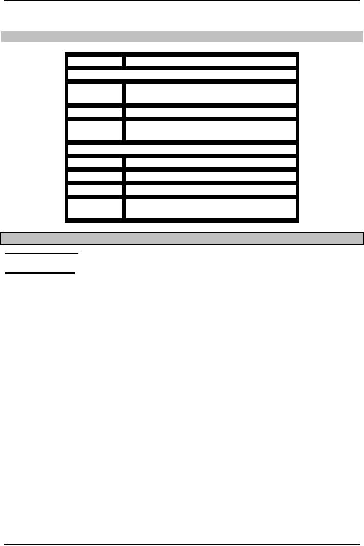
Aggregate Planning Relationships

Type of Costs

How to Calculate

Output

Regular

Regular Cost per Unit X Quantity of Regular

Output

Overtime

Overtime Cost per Unit X Overtime Quantity

Subcontract

Subcontract Cost per Unit X Subcontract

Quantity

Hire/Layoff

Hire

Cost Per Hire X Number Hired

Layoff

Cost per Layoff X Number laid off

Inventory

Carrying Cost per Unit X Average Inventory

Back Order

Back Order Cost Per Unit X Number of

Backorder Units

Mathematical Techniques

Linear programming: Methods for obtaining optimal solutions to problems involving allocation of

scarce resources in terms of cost minimization.

Linear decision rule: Optimizing technique that seeks to minimize combined costs, using a set of cost-

approximating functions to obtain a single quadratic equation.

140

Production and Operations Management MGT613

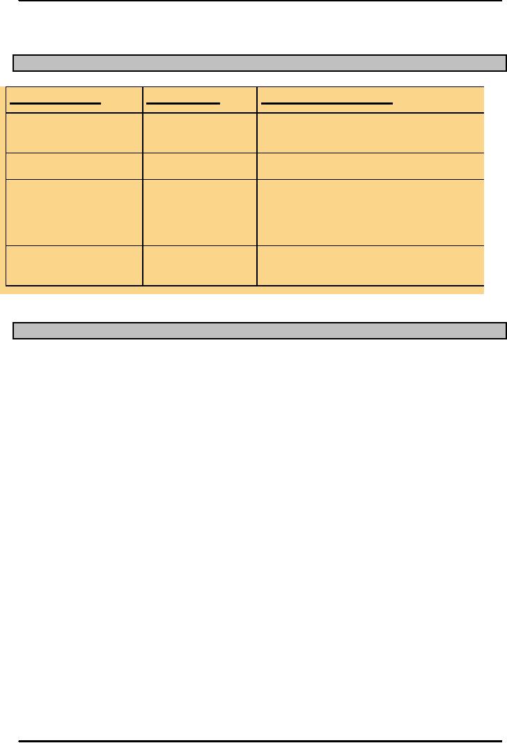
Summary of Planning Techniques

Technique

Solution

Characteristics

Graphical/charting

Trial and

Intuitively appealing, easy to

error

understand; solution not

necessarily optimal.

Linear

Optimizing

Computerized; linear assumptions

not always valid.

programming

Linear

Optimizing

Complex, requires considerable

decision rule

effort to obtain pertinent cost

information and to construct

model; cost assumptions not

always valid.

Simulation

Trial and

Computerized models can be

error

examined under a variety of

conditions.

Aggregate Planning in Services

1. Services occur when they are rendered .Unlike most manufacturing output, most services cannot

be inventoried. Services such as financial planning, tax counseling and oil changes cant be

inventoried/stockpiled. This removes the option of building up the inventories during a slow

period in anticipation of future demand.

2. Demand for service can be difficult to predict .The volume of demand for services is often

variable. In some situations, customers may need prompt service . e.g. police, fire, medical

emergency while in others they may not need prompt service and may be willing to find some

other service provider.

3. Capacity Availability can be difficult to predict. Processing requirements for services can

sometimes be quite variable, similar to the variability of work in a job shop setting.

4. Demand for service can be difficult to predict It is difficult to measure the capacity of a person

rendering a service, a dentist, a Montessorian, a bank teller in anticipation of future demand).

5. Labor Flexibility can be advantage in Services Labor often comprises a significant portion of

service compared to manufacturing. That coupled with the fact that service providers are often

able to handle a fairly wide variety of service requirements means that to some extent, planning

is easier than manufacturing

141

Production and Operations Management MGT613

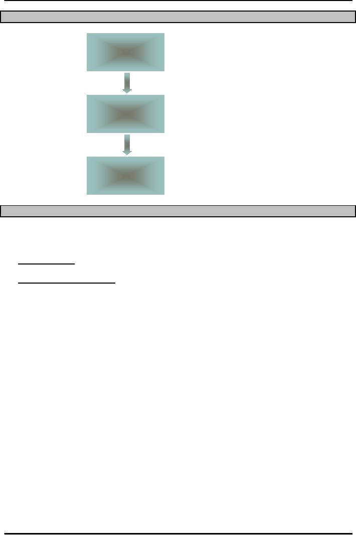
Aggregate Plan to Master Schedule

Aggregat

Dissaggregatio

Master

Schedul

Disaggregating the Aggregate Plan

The Aggregate Plan is broken down into Master Schedules and Rough Cut Capacity Planning charts

respectively.

Master schedule: The result of disaggregating an aggregate plan; shows quantity and timing of

specific end items for a scheduled horizon.

Rough-cut capacity planning: Approximate balancing of capacity and demand to test the feasibility

of a master schedule.

WE WILL DISCUSS IT IN DETAIL WHEN WE COVER OUR MRP LECTURE

E.g. Suppose the organization is making 500 aggregate units of Air conditioners for the month of

March and April with breakup being 200 for window types, 300 type split units with further tonnage

capacities.

A master schedule shows the planned output for individual products rather than an entire product

group, along with the timing of production.

With Rough cut capacity planning we can check capacities of production and warehouses

constraints exist. This means checking capacities of production and warehouse facilities, labor and

vendors to ensure that no gross deficiencies exist that will render master schedule unworkable. The

master schedule then serves as the basis for short range planning.

MS is disaggregated in stages or phases, which may cover weeks or months.

Master schedule: Determines quantities needed to meet demand

Interfaces with

1. Marketing

2. Capacity planning

3. Production planning

4. Distribution planning

142

Production and Operations Management MGT613

Master Scheduling

A Master schedule indicates the quantity and timing ( i.e. delivery times) for a product, or a group

of products, but it does not show planned production. For a master schedule may call for delivery of

500 Air conditioners on April 1. But it may not require any production because of availability of

1000 air conditioners in inventory. Or if there are only 400 Air conditioners, 100 would be planned

for production.

Master Scheduler

Evaluates impact of new orders

Provides delivery dates for orders

Deals with problems

Production delays

Revising master schedule

Insufficient capacity

Projected On-hand Inventory

Projected on-hand

Inventory from

Current week's

inventory

previous week

requirements

Stabilizing the Master Schedule

Changes to a master schedule can be disruptive, particularly changes to the early, or near, portions

of the schedule.

Typically the further out in the future a change is, the less the tendency to cause problems.

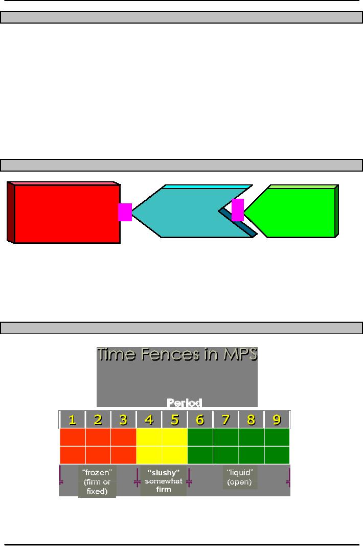
Master Production Schedules are often divided into 4 stages or phases. The dividing lines between

phases are sometimes referred to as time fences.

Time Fences in MPS

In the first phase, usually the first few periods of the schedule, changes can be quite disruptive.

143

Production and Operations Management MGT613

Consequently, once established, that portion of the schedule is generally frozen, which implies that

all but the most critical changes cannot be made without permission from the highest levels in an

organization. This helps in achieving high degree of stability in the production system.

In the next stage, perhaps the next two days or three periods, changes are still disruptive, but not to

that extent that they are in first phase.

Management views the schedule as firm and only exceptional changes are made which helps an

organization gain some competitive advantage.

In the third stage, management views the schedule as full, meaning that all available capacity has

been allocated.

Although changes do impact the schedule, their effect is less dramatic and they are usually made if

there is good reason for doing so.

IN the final phase, management views the schedule as open, meaning that not all capacity has been

allocated. This is where new orders are usually in the Schedule.

144

Table of Contents: