 |
Production
and Operations Management
MGT613
VU
Lesson
10
The
formula for the moving
average is:
Ft = w
1A t -1
+ w 2 A
t - 2 + w 3 A
t -3 + ... + w n
A t -n
n
∑w
=1
wt =
weight given to time period
"t" occurrence (weights must
add to one)
i
i=1
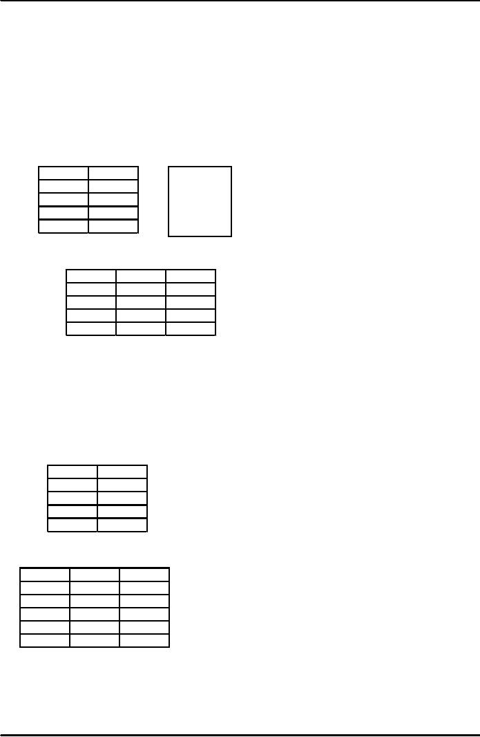
Weighted
Moving Average Problem (1)
Data
Question:
Given the weekly demand and
weights, what is the
forecast for the 4th
period or
Week
4?
Week
Demand
Weights:
1
650
t-1
.5
2
678
t-2
.3
3
720
t-3
.2
4
Weighted
Moving Average Problem (1)
Solution
Week
Demand
Forecast
1
650
2
678
3
720
4
693.4
F4
= 0.5(720)+0.3(678)+0.2(650)=693.4
Note:
More weight age would be given to recent
most values.
Weighted
Moving Average Problem (2)
Data
Question:
Given the weekly demand
information and weights, what is
the weighted moving
average
forecast of the 5th period
or week?
Week
Demand
Weights:
1
820
t-1
0.7
2
775
t-2
0.2
3
680
t-3
0.1
4
655
Weighted
Moving Average Problem (2)
Solution
Week
Demand
Forecast
1
820
2
775
3
680
4
655
5
672
40
Production
and Operations Management
MGT613
VU
F5
= (0.1)(755)+(0.2)(680)+(0.7)(655)= 672
Note:
More weight age would be given to recent
most values.
Exponential
Smoothing Model
Ft =
Ft-1 + a(At-1 -
Ft-1)
Where:
Ft =
Forcast vaue
for thecomingt
timeperiod
l
Ft - 1 =
Forecast
v luein 1 past
timeperiod
a
At - 1 =
Actualoccurancein
thepast t tim
period
e
α
= Alphasmoothingconstant
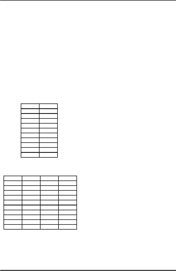
Exponential
Smoothing Problem (1)
Data
Question:
Given the weekly demand data, what
are the exponential smoothing
forecasts
for
periods 2-10 using a=0.10
and a=0.60?
Assume
F1=D1
Week
Demand
1
820
2
775
3
680
4
655
5
750
6
802
7
798
8
689
9
775
10
Exponential
Smoothing Solution
(1)
Week
Demand
0.1
0.6
1
820
820.00
820.00
2
775
820.00
820.00
3
680
815.50
820.00
4
655
801.95
817.30
5
750
787.26
808.09
6
802
783.53
795.59
7
798
785.38
788.35
8
689
786.64
786.57
9
775
776.88
786.61
10
776.69
780.77
41
Production
and Operations Management
MGT613
VU
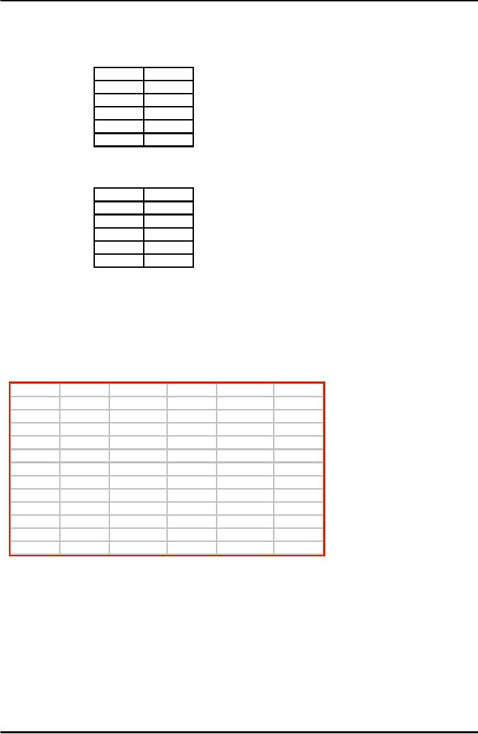
Exponential
Smoothing Problem (2)
Data
Question:
What are the exponential smoothing
forecasts for periods 2-5
using Alpha
=0.5?
Assume F1=D1
Week
Demand
1
820
2
775
3
680
4
655
5
Exponential
Smoothing Problem (2)
Solution
Week
Demand
1
820
2
775
3
680
4
655
5
F1=820+(0.5)(820-820)=820
F3=820+(0.5)(775-820)=797.75
Example
3 - Exponential Smoothing
Period
Actual
Alpha
= 0.1 Error
Alpha
= 0.4 Error
1
42
2
40
42
-2.00
42
-2
3
43
41.8
1.20
41.2
1.8
4
40
41.92
-1.92
41.92
-1.92
5
41
41.73
-0.73
41.15
-0.15
6
39
41.66
-2.66
41.09
-2.09
7
46
41.39
4.61
40.25
5.75
8
44
41.85
2.15
42.55
1.45
9
45
42.07
2.93
43.13
1.87
10
38
42.36
-4.36
43.88
-5.88
11
40
41.92
-1.92
41.53
-1.53
12
41.73
40.92
42

Production
and Operations Management
MGT613
VU
Common
Nonlinear Trends
Parabolic
Exponential
Growth
·
Parabolic Trends
·
Concaved
Upwards and Concaved
Downwards
The
left and right arms are
widening as the value
increases or the parabola is
·
opening
upwards.
It
represents the quadratic
function
·
Linear
Trend Equation
Ft = a +
bt
Where:
·
Ft =
Forecast for period t
·
t =
Specified number of time
periods
·
a =
Value of Ft at t = 0
·
b = Slope of
the line
n
∑
(ty)
-
∑
t∑
y
b=
n∑ t 2
- ∑
t 2
y
-
∑t
a= ∑
n
43

Production
and Operations Management
MGT613
VU
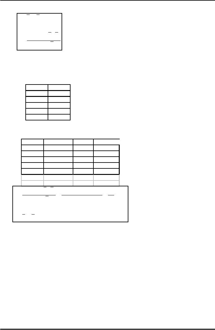
Linear
Trend Equation Example
y
2
Week
t
Sales
ty
1
1
150
150
2
4
157
314
3
9
162
486
4
16
166
664
5
25
177
885
Σ
t2
= 55 Σ y = 812 Σ ty
Σ
t =
15
=
2499
(Σ t)2
=
225
Linear
Trend Calculation
5
(2499) - 15(812)
12495
-12180
b=
=
=
6.3
5(55)
- 225
275
-225
812
- 6.3(15)
a=
=
143.
5
y
= 143.5 + 6.3t
Associative
Forecasting
1.
Predictor
variables -
used to predict values of
variable interest
2.
Regression
-
technique for fitting a line
to a set of points
3.
Least
squares line -
minimizes sum of squared
deviations around the
line
Forecast
Accuracy
·
Error
- difference between actual
value and predicted
value
·
Mean
Absolute Deviation
(MAD)
·
Average
absolute error
·
Mean
Squared Error (MSE)
·
Average
of squared error
·
Mean
Absolute Percent Error
(MAPE)
·
Average
absolute percent
error
44
Production
and Operations Management
MGT613
VU
Simple
Linear Regression Formulas
for Calculating "a" and
"b"
a
= y - bx
∑
xy
- n( y)(x)
b=
∑
x
- n(x)
2
2
Simple
Linear Regression Problem
Data
Question:
Given the data below,
what is the simple linear
regression model that can be used
to
predict
sales in future
weeks?
Week
Sales
1
150
2
157
3
162
4
166
5
177
Answer:
First,
using the linear regression
formulas, we can compute "a" and
"b"
Week
Week*Week
Sales
Week*Sales
1
1
150
150
2
4
157
314
3
9
162
486
4
16
166
664
5
25
177
885
3
55
162.4
2499
Average
Sum
Average
Sum
∑
xy
- n( y)(x) = 2499 - 5(162.4)(3) =
63 =
6.3
b=
∑
x
- n(x)
55
-
5(9)
2
2
10
a
= y - bx = 162.4 - (6.3)(3) = 143.5
The
resulting regression model
is:
Yt =
143.5 + 6.3x
45
Table of Contents:
- INTRODUCTION TO PRODUCTION AND OPERATIONS MANAGEMENT
- INTRODUCTION TO PRODUCTION AND OPERATIONS MANAGEMENT:Decision Making
- INTRODUCTION TO PRODUCTION AND OPERATIONS MANAGEMENT:Strategy
- INTRODUCTION TO PRODUCTION AND OPERATIONS MANAGEMENT:Service Delivery System
- INTRODUCTION TO PRODUCTION AND OPERATIONS MANAGEMENT:Productivity
- INTRODUCTION TO PRODUCTION AND OPERATIONS MANAGEMENT:The Decision Process
- INTRODUCTION TO PRODUCTION AND OPERATIONS MANAGEMENT:Demand Management
- Roadmap to the Lecture:Fundamental Types of Forecasts, Finer Classification of Forecasts
- Time Series Forecasts:Techniques for Averaging, Simple Moving Average Solution
- The formula for the moving average is:Exponential Smoothing Model, Common Nonlinear Trends
- The formula for the moving average is:Major factors in design strategy
- The formula for the moving average is:Standardization, Mass Customization
- The formula for the moving average is:DESIGN STRATEGIES
- The formula for the moving average is:Measuring Reliability, AVAILABILITY
- The formula for the moving average is:Learning Objectives, Capacity Planning
- The formula for the moving average is:Efficiency and Utilization, Evaluating Alternatives
- The formula for the moving average is:Evaluating Alternatives, Financial Analysis
- PROCESS SELECTION:Types of Operation, Intermittent Processing
- PROCESS SELECTION:Basic Layout Types, Advantages of Product Layout
- PROCESS SELECTION:Cellular Layouts, Facilities Layouts, Importance of Layout Decisions
- DESIGN OF WORK SYSTEMS:Job Design, Specialization, Methods Analysis
- LOCATION PLANNING AND ANALYSIS:MANAGING GLOBAL OPERATIONS, Regional Factors
- MANAGEMENT OF QUALITY:Dimensions of Quality, Examples of Service Quality
- SERVICE QUALITY:Moments of Truth, Perceived Service Quality, Service Gap Analysis
- TOTAL QUALITY MANAGEMENT:Determinants of Quality, Responsibility for Quality
- TQM QUALITY:Six Sigma Team, PROCESS IMPROVEMENT
- QUALITY CONTROL & QUALITY ASSURANCE:INSPECTION, Control Chart
- ACCEPTANCE SAMPLING:CHOOSING A PLAN, CONSUMERâS AND PRODUCERâS RISK
- AGGREGATE PLANNING:Demand and Capacity Options
- AGGREGATE PLANNING:Aggregate Planning Relationships, Master Scheduling
- INVENTORY MANAGEMENT:Objective of Inventory Control, Inventory Counting Systems
- INVENTORY MANAGEMENT:ABC Classification System, Cycle Counting
- INVENTORY MANAGEMENT:Economic Production Quantity Assumptions
- INVENTORY MANAGEMENT:Independent and Dependent Demand
- INVENTORY MANAGEMENT:Capacity Planning, Manufacturing Resource Planning
- JUST IN TIME PRODUCTION SYSTEMS:Organizational and Operational Strategies
- JUST IN TIME PRODUCTION SYSTEMS:Operational Benefits, Kanban Formula
- JUST IN TIME PRODUCTION SYSTEMS:Secondary Goals, Tiered Supplier Network
- SUPPLY CHAIN MANAGEMENT:Logistics, Distribution Requirements Planning
- SUPPLY CHAIN MANAGEMENT:Supply Chain Benefits and Drawbacks
- SCHEDULING:High-Volume Systems, Load Chart, Hungarian Method
- SEQUENCING:Assumptions to Priority Rules, Scheduling Service Operations
- PROJECT MANAGEMENT:Project Life Cycle, Work Breakdown Structure
- PROJECT MANAGEMENT:Computing Algorithm, Project Crashing, Risk Management
- Waiting Lines:Queuing Analysis, System Characteristics, Priority Model