Planning

<< Introduction to learning

Advanced Topics >>

Artificial Intelligence (CS607)

Location=Airpo

Has radio?=No

Sells

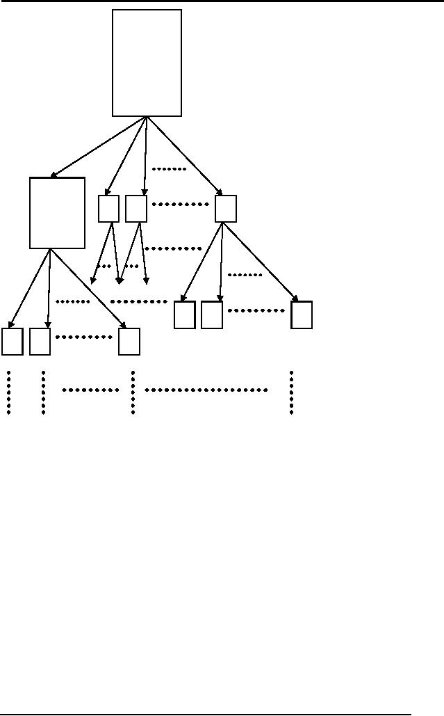
Figure Search space

radio?=No

IsHotel?=No

of a moderate problem

IsMarket?=No

ReservationDo

Although this tree is

ne?=No

just a depiction of

how a search space

grows for realistic

BuyRadio

problems, yet after

TurnRightTurnLeft

seeing this tree we

can

very

well

imagine for even

Location=Airport

Has radio?=No

Sells radio?=No

complex

IsHotel?=No

IsMarket?=No

problems that the

ReservationDone

?=No

search tree could

be too big, big

enough to trouble

us. So the question

is, can we make

such

inefficient

problem solving any

better?

Good news is that

the answer is yes.

How?

Simply

speaking,

this

`search' technique

could be improved

by acting a bit logically instead of blindly. For example not using operators at a

state where their usage is illogical. Like operator `sleeping' should not be even

tried to generate children nodes from a state where I am not at the hotel, or even

haven't reserved the room.

The field of acting logically to solve problems is known as Planning. Planning is

based on logic representation that we have already studied, so you will not find it

too difficult and thus we have kept it short.

8.2 Definition of Planning

The key in planning is to use logic in order to solve problem elegantly. People

working in AI have devised different techniques and algorithms for planning. We

will now introduce a basic definition of planning.

Planning is an advanced form problem solving which generates a sequence of

operators that guarantee the goal. Furthermore, such sequence of operators or

actions (commonly used in planning literature) is called a plan.

196

Artificial Intelligence (CS607)

8.3 Planning vs. problem solving

Planning introduces the following improvements with respect to classical problem

solving:

Each state is represented in predicate logic. De-facto representation of a

state is the conjunction (AND) of predicates that are true in that state.

The goal is also represented as states, i.e. conjunction of predicates.

Each action (or operator) is associated with some logic preconditions that

must be true for that action to be applied. Thus a planning system can

avoid any action that is just not possible at a particular state.

Each action is associated with an `effect' or post-conditions. These post-

conditions specify the added and/or deleted predicates when the action is

applied.

The inference mechanism used is that of backward chaining so as to use

only the actions and states that are really required to reach goal state.

Optional: The sequence of actions (plan) is minimally ordered. Only those

actions are ordered in a sequence when any other order will not achieve

the desired goal. Therefore, planning allows partial ordering i.e. there can

be two actions that are not in any order from each other because any

particular order used amongst them will achieve the same goal.

8.4 Planning language

STRIPS is one of the founding languages developed particularly for planning. Let

us understand planning to a better level by seeing what a planning language can

represent.

8.4.1 Condition predicates

Condition predicates are the predicates that define states. For example, a

predicate that specifies that we are at location `X' is given as.

at(X)

8.4.2 State

State is a conjunction of predicates represented in well-known form, for example,

a state where we are at the hotel and do not have either cash or radio is

represented as,

at(hotel) ∧ ¬have(cash) ∧ ¬have(radio)

8.4.3 Goal

Goal is also represented in the same manner as a state. For example, if the goal

of a planning problem is to be at the hotel with radio, it is represented as,

197

Artificial Intelligence (CS607)

at(hotel) ∧ have(radio)

8.4.4 Action Predicates

Action is a predicate used to change states. It has three components namely, the

predicate itself, the pre-condition, and post-condition predicates. For example,

the action to buy something item can be represented as,

Action:

buy(X)

Pre-conditions:

at(Place) ∧ sells(Place, X)

Post-conditions/Effect:

have(X)

What this example action says is that to buy any item `X', you have to be (pre-

conditions) at a place `Place' where `X' is sold. And when you apply this operator

i.e. buy `X', then the consequence would be that you have item `X' (post-

conditions).

8.5 The partial-order planning algorithm POP

Now that we know what planning is and how states and actions are represented,

let us see a basic planning algorithm POP.

POP(initial_state, goal, actions) returns plan

Begin

Initialize plan `p' with initial_state linked to goal state with two

special actions, start and finish

Loop until there is not unsatisfied pre-condition

Find an action `a' which satisfies an unachieved pre-condition of

some action `b' in the plan

Insert `a' in plan linked with `b'

Reorder actions to resolve any threats

End

If you think over this algorithm, it is quite simple. You just start with an empty plan

in which naturally, no condition predicate of goal state is met i.e. pre-conditions of

finish action are not met. You backtrack by adding actions that meet these

unsatisfied pre-condition predicates. New unsatisfied preconditions will be

generated for each newly added action. Then you try to satisfy those by using

appropriate actions in the same way as was done for goal state initially. You keep

on doing that until there is no unsatisfied precondition.

Now, at some time there might be two actions at the same level of ordering of

them one action's effect conflicts with other action's pre-condition. This is called a

198

Artificial Intelligence (CS607)

threat and should be resolved. Threats are resolved by simply reordering such

actions such that you see no threat.

Because this algorithm does not order actions unless absolutely necessary it is

known as a partial-order planning algorithm.

Let us understand it more by means of the example we discussed in the lecture

from [??].

8.6 POP Example

The problem to solve is of shopping a banana, milk and drill from the market and

coming back to home. Before going into the dry-run of POP let us reproduce the

predicates.

The condition predicates are:

At(x)

Has (x)

Sells (s, g)

Path (s, d)

The initial state and the goal state for our algorithm are formally specified as

under.

Initial State:

At(Home) ∧ Sells (HWS, Drill) ∧ Sells (SM, Banana) ∧ Sells (SM, Milk) ∧

Path (home, SM) ∧ path (SM, HWS) ∧ Path (home, HWS)

Goal State:

At (Home) ∧ Has (Banana) ∧ Has (Milk) ∧ Has (Drill)

The actions for this problem are only two i.e. buy and go. We have added the

special actions start and finish for our POP algorithm to work. The definitions for

these four actions are.

Go (x)

Preconditions: at(y) ∧ path(y,x)

Postconditions: at(x) ∧ ~at(y)

Buy (x)

Preconditions: at(s) ∧ sells (s, x)

Postconditions: has(x)

Start ()

Preconditions: nill

Postconditions: At(Home) ∧ Sells (HWS, Drill) ∧ Sells (SM, Banana) ∧

Sells (SM, Milk) ∧ Path (home, SM) ∧ path (SM, HWS) ∧ Path (home, HWS)

Finish ()

Preconditions: At (Home) ∧ Has (Banana) ∧ Has (Milk) ∧ Has (Drill)

199

Artificial Intelligence (CS607)

Postconditions: nill

Note the post-condition of the start action is exactly our initial state. That is how

we have made sure that our end plan starts with the initial state configuration

given. Similarly note that the pre-conditions of finish action are exactly the same

as the goal state. Thus we can ensure that this plan satisfies all the conditions of

the goal state. Also note that naturally there is no pre-condition to start and no

post-condition for finish actions.

Now we start the algorithm by just putting the start and finish actions in our plan

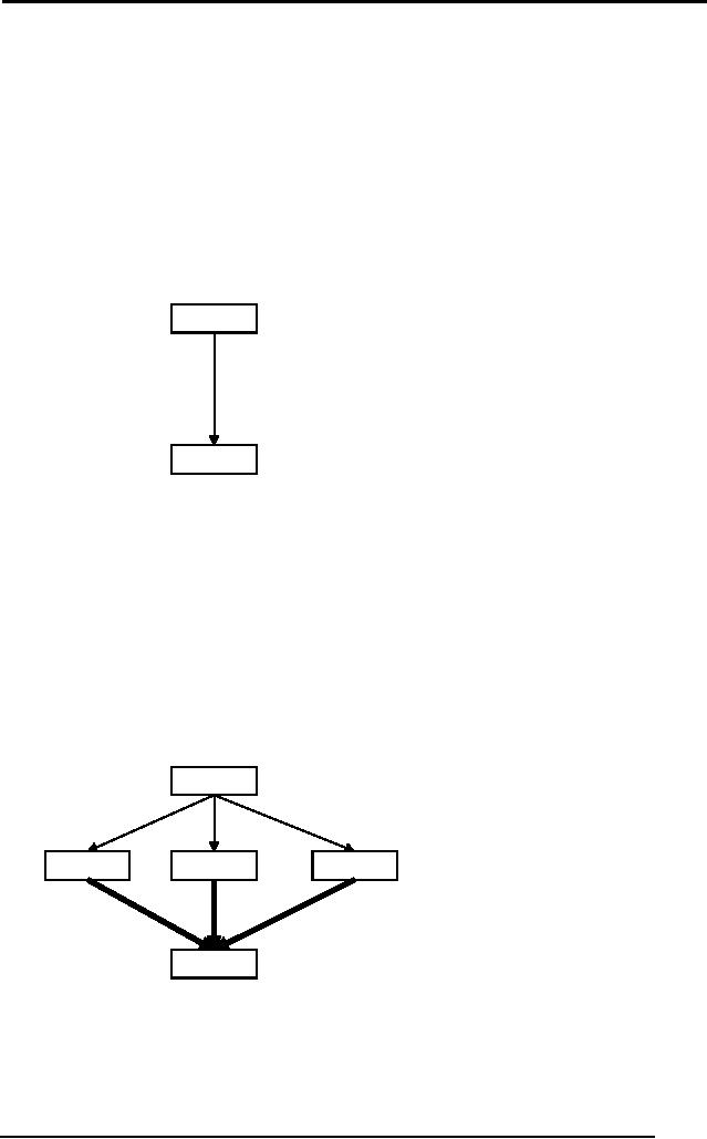
and linking them. After this first initial step the situation becomes as follows.

Start

At(Home) Sells(SM, Banana) Sells(SM, Milk) Sells(HWS, Drill)

Have(Drill) Have(Milk)

Have(Banana) At(Home)

Finish

Figure Initial plan scene A

We now enter the main loop of POP algorithm where we iteratively find any

unsatisfied pre-condition in our existing plan and then satisfying it by an

appropriate action.

At first you see three unsatisfied predicates Have(Drill), Have(Milk) and

Have(Banana). Lets take Have(Drill) first. Have(Drill) matches the post-condition

Have(X) of action Buy(X), where X becomes Drill in this case. Similarly we can

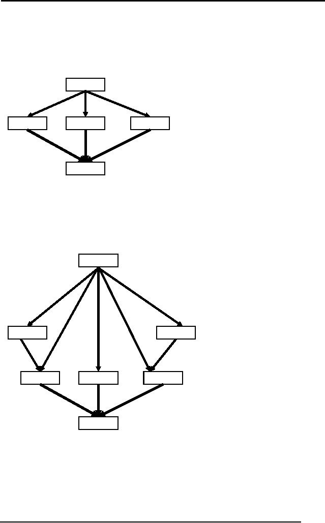
satisfy the other two condition predicates and the resulting plan has three new

actions added as shown below.

Start

Figure Plan scene B

At(s) Sells(s, Drill)

At(s) Sells(s, Milk)

At(s), Sells(s, Bananas)

There is no threat

Buy(Milk)

Buy(Bananas)

Buy(Drill)

visible in the current

plan, so no re-ordering

is required.

Have(Drill), Have(Milk), Have(Bananas) At(Home)

At(Home) Sells(SM, Banana) Sells(SM, Milk) Sells(HWS, Drill)

The algorithm moves

Finish

forward. Now if you see

the Sells() pre-conditions of the three new actions, they are satisfied with the

post-conditions Sells(HWS,Drill), Sells(SM,Banana), and Sells(SM,Milk) of the

Start() action with the exact values as shown.

200

Artificial Intelligence (CS607)

Start

At(HWS), Sells(HWS, Drill)

At(SM), Sells(SM, Milk)

At(SM), Sells(SM, Bananas)

Buy(Milk)

Buy(Bananas)

Buy(Drill)

Have(Drill), Have(Milk), Have(Bananas) At(Home)

Finish

Figure Plan scene C

We now move forward and see what other pre-conditions are not satisfied.

At(HWS) is not satisfied in action Buy(Drill). Similarly At(SM) is not satisfied in

actions Buy(Milk) and Buy(Banana). Only action Go() has post-conditions that

can satisfy these pre-conditions. Adding them one-by-one to satisfy all these pre-

conditions our plan becomes,

Start

Figure Plan scene

Now if we check

for threats we

At(Home)

find that if we go

to HWS from

Go(HWS)

Go(SM)

Home we cannot

go to SM from

Home. Meaning,

At(HWS), Sells(HWS, Drill)

At(SM), Sells(SM, Milk)

At(SM), Sells(SM, Bananas)

post-condition of

Buy(Milk)

Buy(Bananas)

Buy(Drill)

Go(HWS)

threats the pre-

condition

Have(Drill), Have(Milk), Have(Bananas) At(Home)

At(Home)

Go(SM) and vice

Finish

versa. So as

given in our POP algorithm, we have to resolve the threat by reordering these

actions such that no action threat pre-conditions of other action.

That is how POP proceeds by adding actions to satisfy preconditions and

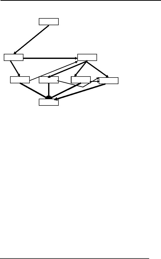
reordering actions to resolve any threat in the plan. The final plan using this

algorithm becomes.

201

Artificial Intelligence (CS607)

Start

Figure Plan scene

You can see

how reordering

At(Home)

is done from this

illustration. For

Go(HWS)

Go(SM)

example

the

threat

observed

At(HWS), Sells(HWS, Drill)

At(SM), Sells(SM, Milk)

At(SM), Sells(SM, Bananas)

between

Buy(Milk)

Buy(Bananas)

Buy(Drill)

Go(Home)

Go(HWS)

and

Go(SM), the link

from Start to

Have(Drill), Have(Milk), Have(Bananas) At(Home)

Go(SM)

has

been

deleted

Finish

and a new links

have been established from Go(HWS) and Buy(Drill) to Go(SM).

To feel more comfortable on the plan we have achieved from this problem, lets

narrate our solution in plain English.

"Start by going to hardware store. Then you can buy drill and then go to the super

market. At the super market, buy milk and banana in any order and then go

home. You are done."

8.7 Problems

1. A Farmer has a tiger, a goat and a bundle of grass. He is standing at one

side of the river with a very week boat which can hold only one of his

belongings at a time. His goal is has to take all three of his belongings to

the other side. The constraint is that the farmer cannot leave either goat

and tiger, or goat and grass, at any side of the river unattended because

one of them will eat the other. Using the simple POP algorithm we studied

in the lecture, solve this problem. Show all the intermediate and final plans

step by step.

2. A robot has three slots available to put the blocks A, B, C. The blocks are

initially placed at slot 1, one upon the other (A placed on B placed on C)

and it's goal is to move all three to slot 3 in the same order. The constraint

to this robot is that it can only move one block from any slot to any other

slot, and it can only pick the top most block from a slot to move. Using the

simple POP algorithm we studied in the lecture, solve this problem. Show

all the intermediate and final plans step by step.

202

Table of Contents: