Problem Solving

<< Introduction

Genetic Algorithms >>

Artificial Intelligence (CS607)

Lecture No. 4 -10

2 Problem Solving

In chapter one, we discussed a few factors that demonstrate intelligence.

Problem solving was one of them when we referred to it using the examples of a

mouse searching a maze and the next number in the sequence problem.

Historically people viewed the phenomena of intelligence as strongly related to

problem solving. They used to think that the person who is able to solve more

and more problems is more intelligent than others.

In order to understand how exactly problem solving contributes to intelligence, we

need to find out how intelligent species solve problems.

2.1 Classical Approach

The classical approach to solving a problem is pretty simple. Given a problem at

hand use hit and trial method to check for various solutions to that problem.

This hit and trial approach usually works well for trivial problems and is referred to

as the classical approach to problem solving.

Consider the maze searching problem. The mouse travels though one path and

finds that the path leads to a dead end, it then back tracks somewhat and goes

along some other path and again finds that there is no way to proceed. It goes on

performing such search, trying different solutions to solve the problem until a

sequence of turns in the maze takes it to the cheese. Hence, of all the solutions

the mouse tries, the one that reached the cheese was the one that solved the

problem.

Consider that a toddler is to switch on the light in a dark room. He sees the

switchboard having a number of buttons on it. He presses one, nothing happens,

he presses the second one, the fan gets on, he goes on trying different buttons till

at last the room gets lighted and his problem gets solved.

Consider another situation when we have to open a combinational lock of a

briefcase. It is a lock which probably most of you would have seen where we

have different numbers and we adjust the individual dials/digits to obtain a

combination that opens the lock. However, if we don't know the correct

combination of digits that open the lock, we usually try 0-0-0, 7-7-7, 7-8-6 or any

such combination for opening the lock. We are solving this problem in the same

manner as the toddler did in the light switch example.

All this discussion has one thing in common. That different intelligent species use

a similar approach to solve the problem at hand. This approach is essentially the

classical way in which intelligent species solve problems. Technically we call this

hit and trial approach the "Generate and Test" approach.

2.2 Generate and Test

This is a technical name given to the classical way of solving problems where we

generate different combinations to solve our problem, and the one which solves

the problem is taken as the correct solution. The rest of the combinations that we

try are considered as incorrect solutions and hence are destroyed.

Artificial Intelligence (CS607)

Possible

Tester

Correct

Solutions

Solution

Generator

Incorrect

Solutions

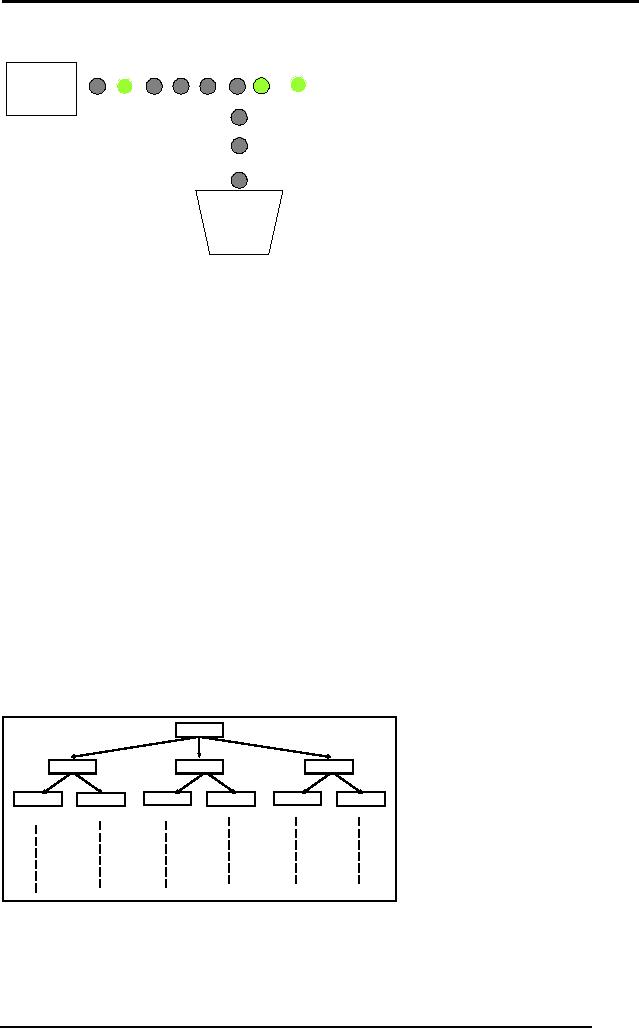
The diagram above shows a simple arrangement of a Generate and Test

procedure. The box on the left labeled "Solution Generator" generates different

solutions to a problem at hand, e.g. in the case of maze searching problem, the

solution generator can be thought of as a machine that generates different paths

inside a maze. The "Tester" actually checks that either a possible solution from

the solution generates solves out problem or not. Again in case of maze

searching the tester can be thought of as a device that checks that a path is a

valid path for the mouse to reach the cheese. In case the tester verifies the

solution to be a valid path, the solution is taken to be the "Correct Solution". On

the other hand if the solution was incorrect, it is discarded as being an "Incorrect

Solution".

2.3 Problem Representation

All the problems that we have seen till now were trivial in nature. When the

magnitude of the problem increases and more parameters are added, e.g. the

problem of developing a time table, then we have to come up with procedures

better than simple Generate and Test approach.

Before even thinking of developing techniques to systematically solve the

problem, we need to know one more thing that is true about problem solving

namely problem representation. The key to problem solving is actually good

representation of a problem. Natural representation of problems is usually done

using graphics and diagrams to develop a clear picture of the problem in your

mind. As an example to our comment consider the diagram below.

OFF | OFF | OFF

OFF

ON | OFF | OFF

OFF | ON | OFF

OFF | OFF | ON

ON | ON | OFF

ON | OFF | ON

OFF | ON | ON

ON | ON | OFF

ON | OFF | ON

It shows the problem of switching on the light by a toddler in a graphical form.

Each rectangle represents the state of the switch board. OFF | OFF| OFF means

that all the three switches are OFF. Similarly OFF| ON | OFF means that the first

and the last switch is OFF and the middle one is ON. Starting from the state

when all the switches are OFF the child can proceed in any of the three ways by

Artificial Intelligence (CS607)

switching either one of the switch ON. This brings the toddler to the next level in

the tree. Now from here he can explore the other options, till he gets to a state

where the switch corresponding to the light is ON. Hence our problem was

reduced to finding a node in the tree which ON is the place corresponding to the

light switch. Observe how representing a problem in a nice manner clarifies the

approach to be taken in order to solve it.

2.4 Components of Problem Solving

Let us now be a bit more formal in dealing with problem solving and take a look at

the topic with reference to some components that constitute problem solving.

They are namely: Problem Statement, Goal State, Solution Space and Operators.

We will discuss each one of them in detail.

2.4.1 Problem Statement

This is the very essential component where by we get to know what exactly the

problem at hand is. The two major things that we get to know about the problem

is the Information about what is to be done and constraints to which our solution

should comply. For example we might just say that given infinite amount of time,

one will be able to solve any problem he wishes to solve. But the constraint

"infinite amount of time" is not a practical one. Hence whenever addressing a

problem we have to see that how much time shall out solution take at max. Time

is not the only constraint. Availability of resources, and all the other parameters

laid down in the problem statement actually tells us about all the rules that have

to be followed while solving a problem. For example, taking the same example of

the mouse, are problem statement will tell us things like, the mouse has to reach

the cheese as soon as possible and in case it is unable to find a path within an

hour, it might die of hunger. The statement might as well tell us that the mouse is

located in the lower left corner of the maze and the cheese in the top left corner,

the mouse can turn left, right and might or might not be allowed to move

backward and things like that. Thus it is the problem statement that gives us a

feel of what exactly to do and helps us start thinking of how exactly things will

work in the solution.

2.4.2 Problem Solution

While solving a problem, this should be known that what will be out ultimate aim.

That is what should be the output of our procedure in order to solve the problem.

For example in the case of mouse, the ultimate aim is to reach the cheese. The

state of world when mouse will be beside the cheese and probably eating it

defines the aim. This state of world is also referred to as the Goal State or the

state that represents the solution of the problem.

2.4.3 Solution space

In order to reach the solution we need to check various strategies. We might or

might not follow a systematic strategy in all the cases. Whatever we follow, we

have to go though a certain amount of states of nature to reach the solution. For

example when the mouse was in the lower left corner of the maze, represents a

state i.e. the start state. When it was stuck in some corner of the maze

represents a state. When it was stuck somewhere else represents another state.

When it was traveling on a path represents some other state and finally when it

Artificial Intelligence (CS607)

reaches the cheese represents a state called the goal state. The set of the start

state, the goal state and all the intermediate states constitutes something which

is called a solution space.

2.4.4 Traveling in the solution space

We have to travel inside this solution space in order to find a solution to our

problem. The traveling inside a solution space requires something called as

"operators". In case of the mouse example, turn left, turn right, go straight are

the operators which help us travel inside the solution space. In short the action

that takes us from one state to the other is referred to as an operator. So while

solving a problem we should clearly know that what are the operators that we can

use in order to reach the goal state from the starting state. The sequence of

these operators is actually the solution to our problem.

2.5 The Two-One Problem

In order to explain the four components of problem solving in a better way we

have chosen a simple but interesting problem to help you grasp the concepts.

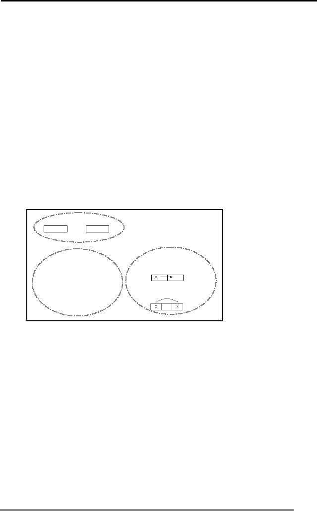
The diagram below shows the setting of our problem called the Two-One

Problem.

Start

Goal

11?22

22?11

Legal Moves:

· Slide

Rules:

· 1s' move right

· 2s' move left

· Hop

· Only one move at a time

· No backing up

A simple problem statement to the problem at hand is as under.

You are given a rectangular container that has 5 slots in it. Each slot can hold

only one coin at a time. Place Rs.1 coins in the two left slots; keep the center slot

empty and put Rs.2 coins in the two right slots. A simple representation can be

seen in the diagram above where the top left container represents the Start State

in which the coined are placed as just described. Our aim is to reach a state of

the container where the left two slots should contain Rs.2 coins, the center slot

should be empty and the right two slots should contain Rs.1 coin as shown in the

Goal State. There are certain simple rules to play this game. The rules are

mentioned clearly in the diagram under the heading of "Rules". The rules actually

define the constraints under which the problem has to be solved. The legal

moves are the Operators that we can use to get from one state to the other. For

example we can slide a coin to its left or right if the left or right slot is empty, or

we can hop the coin over a single slot. The rules say that Rs.1 coins can slide or

hop only towards right. Similarly the Rs.2 coins can slide or hop only towards the

left. You can only move one coin at a time.

Artificial Intelligence (CS607)

Now let us try to solve the problem in a trivial manner just by using a hit and trial

method without addressing the problem in a systematic manner.

Trial 1

Start State

Move 1

Move 2

Move 3

Move 4

Move 5

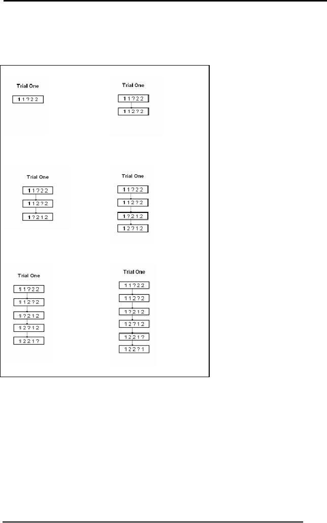
In Move 1 we slide a 2 to the left, then we hop a 1 to the right, then we slide the 2

to the left again and then we hop the 2 to the left, then slide the one to the right

hence at least one 2 and one 1 are at the desired positions as required in the

goal state but then we are stuck. There is no other valid move which takes us out

of this state. Let us consider another trial.

Trial 2

Artificial Intelligence (CS607)

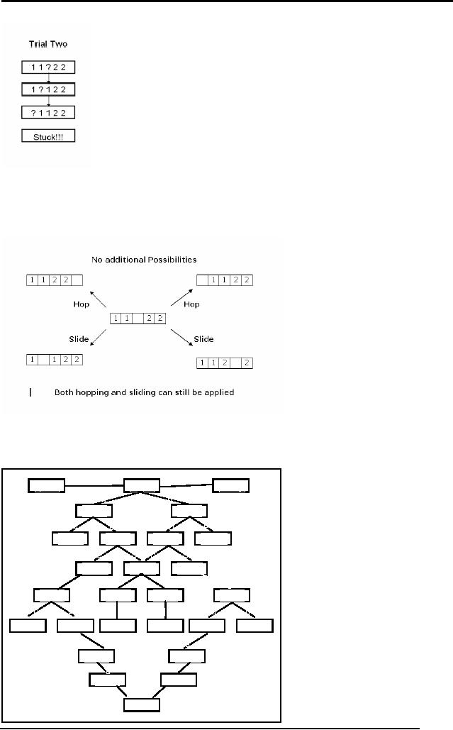
Starting from the start state we first hop a 1 to the right, then we slide the other 1

to the right and then suddenly we get STUCK!! Hence solving the problem

through a hit and trial might not give us the solution.

Let us now try to address the problem in a systematic manner. Consider the

diagram below.

Starting from the goal state if we hop, we get stuck. If we slide we can further

carry on. Keeping this observation in mind let us now try to develop all the

possible combinations that can happen after we slide.

?1122

11?22

1122 ?

1?122

1 1 2? 2

?1122

1 2 1? 2

1?212

1122 ?

1212 ?

12 ?12

?1212

12?21

?2112

1 2 2 1?

21?12

1 2 2? 1

?2121

2?112

1 2 2 ?1

2112 ?

2?112

2?121

212 ?1

2?211

2 2 1? 1

1 1? 2 2

Artificial Intelligence (CS607)

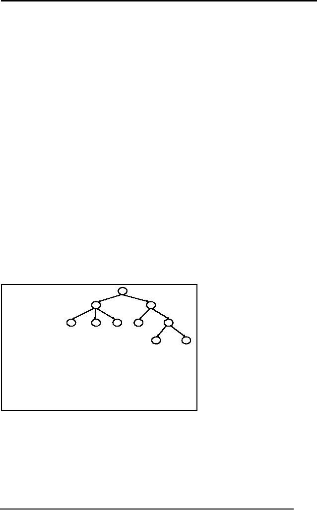
The diagram above shows a tree sort of structure enumerating all the possible

states and moves. Looking at this diagram we can easily figure out the solution to

our problem. This tree like structure actually represents the "Solution Space" of

this problem. The labels on the links are H and S representing hop and slide

operators respectively. Hence H and S are the operators that help us travel

through this solution space in order to reach the goal state from the start state.

We hope that this example actually clarifies the terms problem statement, start

state, goal state, solution space and operators in your mind. It will be a nice

exercise to design your own simple problems and try to identify these

components in them in order to develop a better understanding.

2.6 Searching

All the problems that we have looked at can be converted to a form where we

have to start from a start state and search for a goal state by traveling through a

solution space. Searching is a formal mechanism to explore alternatives.

Most of the solution spaces for problems can be represented in a graph where

nodes represent different states and edges represent the operator which takes us

from one state to the other. If we can get our grips on algorithms that deal with

searching techniques in graphs and trees, we'll be all set to perform problem

solving in an efficient manner.

2.7 Tree and Graphs Terminology

Before studying the searching techniques defined on trees and graphs let us

briefly review some underlying terminology.

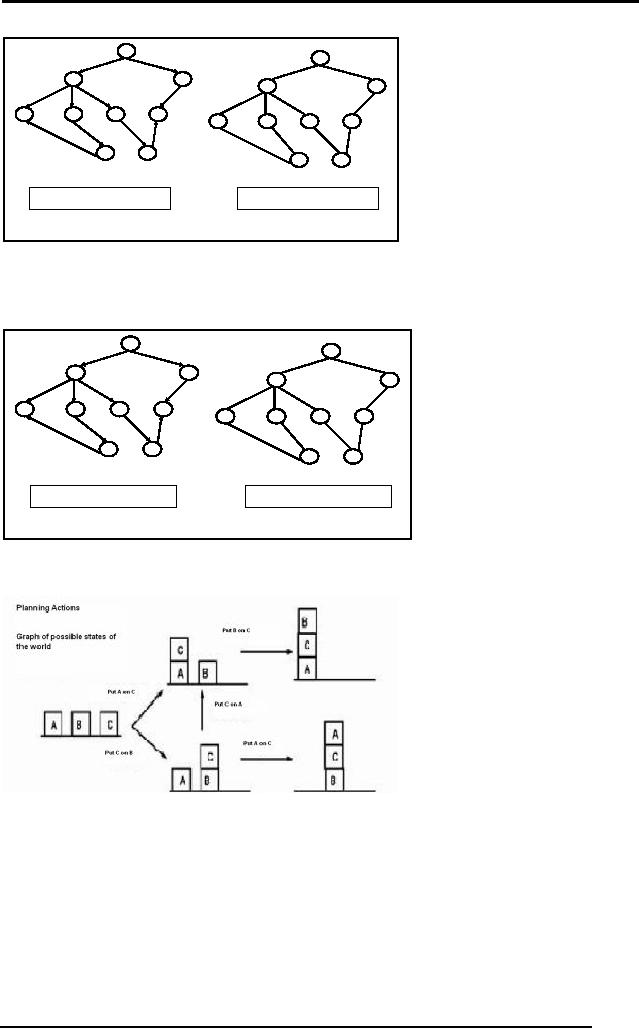
·"A" is the "root node"

·"A, B, C .... J" are "nodes"

·"B" is a "child" of "A"

·"A" is ancestor of "D"

·"D" is a descendant of "A"

·"D, E, F, G, I, J" are "leaf nodes"

·Arrows represent "edges" or "links"

The diagram above is just to refresh your memories on the terminology of a tree.

As for graphs, there are undirected and directed graphs which can be seen in the

diagram below.

Artificial Intelligence (CS607)

Directed Graph

Undirected Graph

Let us first consider a couple of examples to learn how graphs can represent

important information by the help of nodes and edges.

Graphs can be used to represent city routes.

Directed Graph

Undirected Graph

Graphs can be used to plan actions.

We will use graphs to represent problems and their solution spaces. One thing to

be noted is that every graph can be converted into a tree, by replicating the

nodes. Consider the following example.

Artificial Intelligence (CS607)

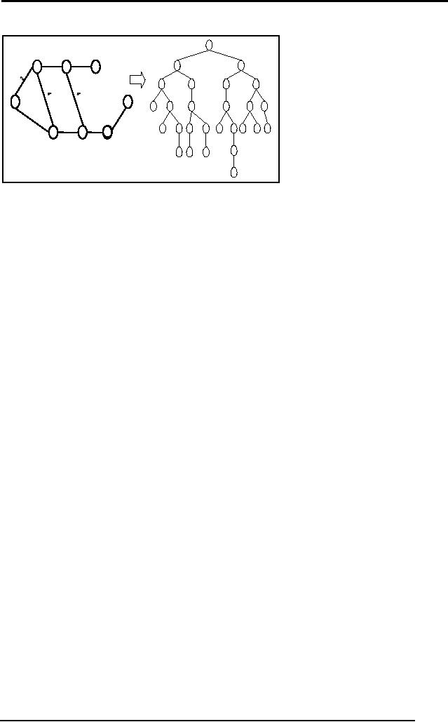
The graph in the figure represents a city map with cities labeled as S, A, B, C, D,

E, F and G. Just by following a simple procedure we can convert this graph to a

tree.

Start from node S and make it the root of your tree, check how many nodes are

adjacent to it. In this case A and D are adjacent to it. Hence in the tree make A

and D, children of S. Now go on proceeding in this manner and you'll get a tree

with a few nodes replicated. In this manner depending on a starting node you can

get a different tree too. But just recall that when solving a problem; we usually

know the start state and the end state. So we will be able to transform our

problem graphs in problem trees. Now if we can develop understanding of

algorithms that are defined for tree searching and tree traversals then we will be

in a better shape to solve problems efficiently.

We know that problems can be represented in graphs, and are well familiar with

the components of problem solving, let us now address problem solving in a

more formal manner and study the searching techniques in detail so that we can

systematically approach the solution to a given problem.

2.8 Search Strategies

Search strategies and algorithms that we will study are primarily of four types,

blind/uninformed, informed/heuristic, any path/non-optimal and optimal path

search algorithms. We will discuss each of these using the same mouse

example.

Suppose the mouse does not know where and how far is the cheese and is

totally blind to the configuration of the maze. The mouse would blindly search the

maze without any hints that will help it turning left or right at any junction. The

mouse will purely use a hit and trial approach and will check all combinations till

one takes it to the cheese. Such searching is called blind or uninformed

searching.

Consider now that the cheese is fresh and the smell of cheese is spread through

the maze. The mouse will now use this smell as a guide, or heuristic (we will

comment on this word in detail later) to guess the position of the cheese and

choose the best from the alternative choices. As the smell gets stronger, the

Artificial Intelligence (CS607)

mouse knows that the cheese is closer. Hence the mouse is informed about the

cheese through the smell and thus performs an informed search in the maze.

For now you might think that the informed search will always give us a better

solution and will always solve our problem. This might not be true as you will find

out when we discuss the word heuristic in detail later.

When solving the maze search problem, we saw that the mouse can reach the

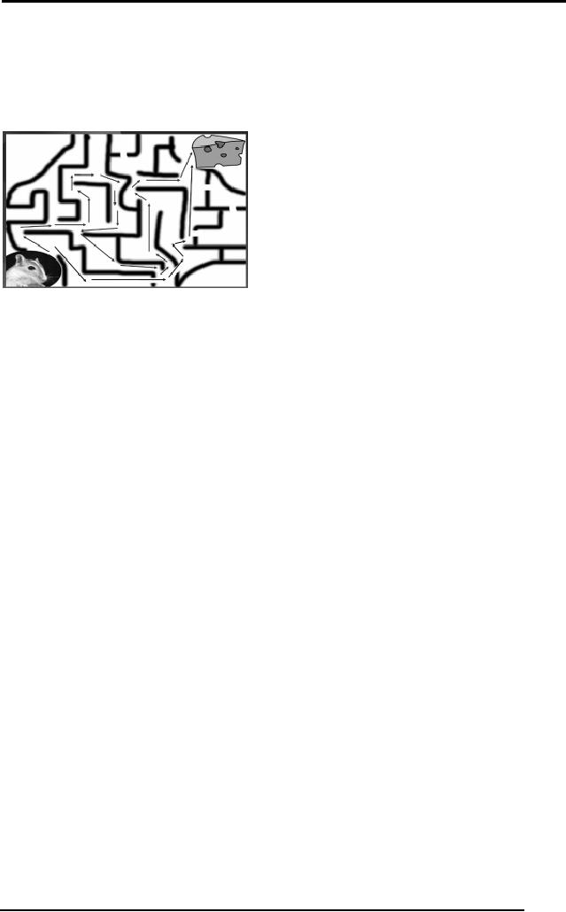
cheese from different paths. In the diagram above two possible paths are shown.

In any-path/non optimal searches we are concerned with finding any one solution

to our problem. As soon as we find a solution, we stop, without thinking that there

might as well be a better way to solve the problem which might take lesser time

or fewer operators.

Contrary to this, in optimal path searches we try to find the best solution. For

example, in the diagram above the optimal path is the blue one because it is

smaller and requires lesser operators. Hence in optimal searches we find

solutions that are least costly, where cost of the solution may be different for

each problem.

2.9 Simple Search Algorithm

Let us now state a simple search algorithm that will try to give you an idea about

the sort of data structures that will be used while searching, and the stop criteria

for your search. The strength of the algorithm is such that we will be able to use

this algorithm for both Depth First Search (DFS) and Breadth First Search (BFS).

Let S be the start state

1. Initialize Q with the start node Q=(S) as the only entry; set Visited =

(S)

2. If Q is empty, fail. Else pick node X from Q

3. If X is a goal, return X, we've reached the goal

4. (Otherwise) Remove X from Q

5. Find all the children of state X not in Visited

6. Add these to Q; Add Children of X to Visited

7. Go to Step 2

Here Q represents a priority queue. The algorithm is simple and doesn't need

much explanation. We will use this algorithm to implement blind and uninformed

searches. The algorithm however can be used to implement informed searches

Artificial Intelligence (CS607)

as well. The critical step in the Simple Search Algorithm is picking of a node X

from Q according to a priority function. Let us call this function P(n). While using

this algorithm for any of the techniques, our priority will be to reduce the value of

P(n) as much as we can. In other words, the node with the highest priority will

have the smallest value of the function P(n) where n is the node referred to as X

in the algorithm.

2.10 Simple Search Algorithm Applied to Depth First Search

Depth First Search dives into a tree deeper and deeper to fine the goal state. We

will use the same Simple Search Algorithm to implement DFS by keeping our

priority function as

P(n) =

height (n)

As mentioned previously we will give priority to the element with minimum P(n)

hence the node with the largest value of height will be at the maximum priority to

be picked from Q. The following sequence of diagrams will show you how DFS

works on a tree using the Simple Search Algorithm.

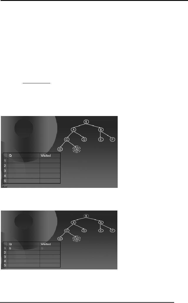
We start with a tree containing nodes S, A, B, C, D, E, F, G, and H, with H as the

goal node. In the bottom left table we show the two queues Q and Visited.

According to the Simple Search Algorithm, we initialize Q with the start node S,

shown below.

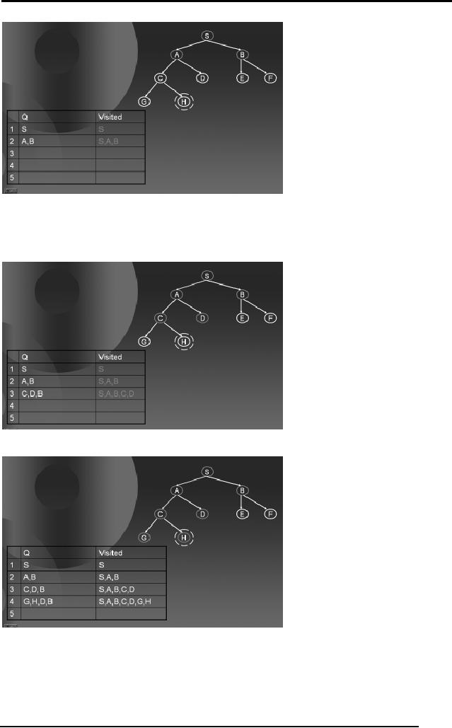
If Q is not empty, pick the node X with the minimum P(n) (in this case S), as it is

the only node in Q. Check if X is goal, (in this case X is not the goal). Hence find

all the children of X not in Visited and add them to Q and Visited. Goto Step 2.

Artificial Intelligence (CS607)

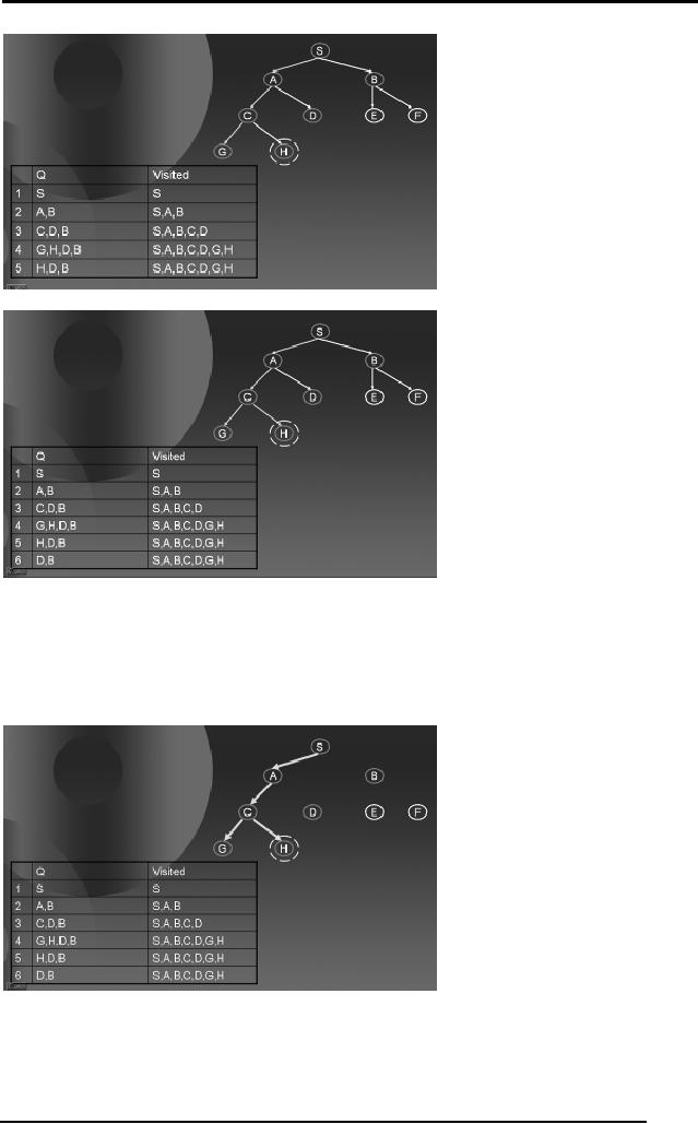
Again check if Q is not empty, pick the node X with the minimum P(n) (in this

case either A or B), as both of them have the same value for P(n). Check if X is

goal, (in this case A is not the goal). Hence, find all the children of A not in Visited

and add them to Q and Visited. Go to Step 2.

Go on following the steps in the Simple Search Algorithm till you find a goal node.

The diagrams below show you how the algorithm proceeds.

Artificial Intelligence (CS607)

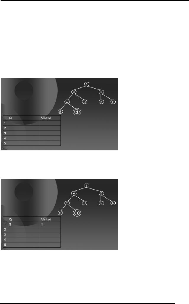
Here, from the 5th row of the table when we remove H and check if it's the goal,

the algorithm says YES and hence we return H as we have reached the goal

state. The path followed by the DFS is shown by green arrows at each step. The

diagram below also shows that DFS didn't have to search the entire search

space, rather only by traveling in half the tree, the algorithm was able to search

the solution.

Hence simply by selecting a specific P(n) our Simple Search Algorithm was

converted to a DFS procedure.

Artificial Intelligence (CS607)

2.11 Simple Search Algorithm Applied to Breadth First Search

Breadth First Search explores the breadth of the tree first and progresses

downward level by level. Now, we will use the same Simple Search Algorithm to

implement BFS by keeping our priority function as

P(n) = height (n)

As mentioned previously, we will give priority to the element with minimum P(n)

hence the node with the largest value of height will be at the maximum priority to

be picked from Q. In other words, greater the depth/height greater the priority.

The following sequence of diagrams will show you how BFS works on a tree

using the Simple Search Algorithm.

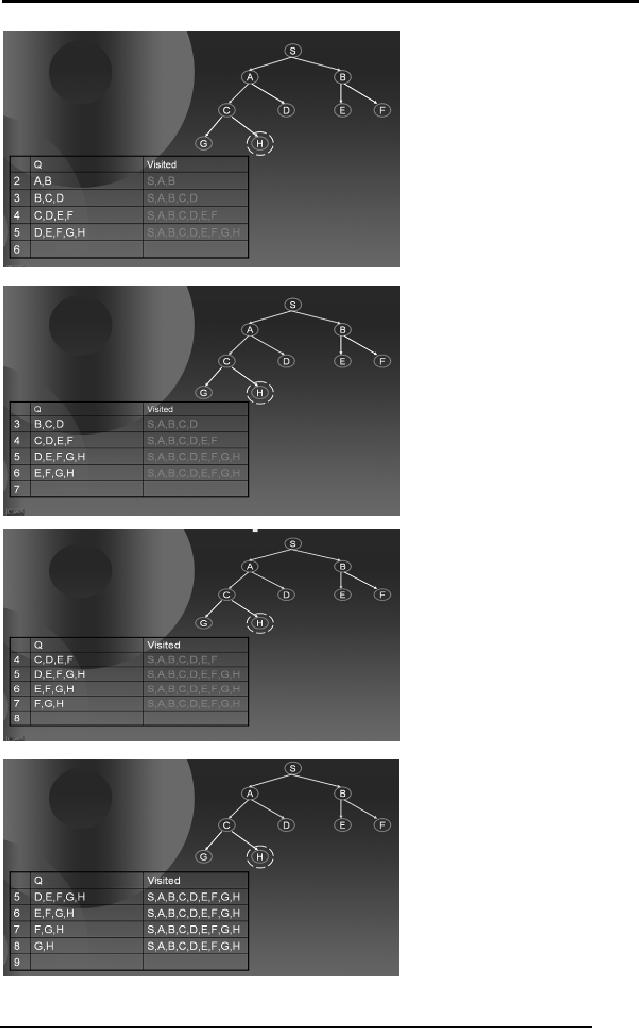
We start with a tree containing nodes S, A, B, C, D, E, F, G, and H, with H as the

goal node. In the bottom left table we show the two queues Q and Visited.

According to the Simple Search Algorithm, we initialize Q with the start node S.

If Q is not empty, pick the node X with the minimum P(n) (in this case S), as it is

the only node in Q. Check if X is goal, (in this case X is not the goal). Hence find

all the children of X not in Visited and add them to Q and Visited. Goto Step 2.

Artificial Intelligence (CS607)

Again, check if Q is not empty, pick the node X with the minimum P(n) (in this

case either A or B), as both of them have the same value for P(n). Remember, n

refers to the node X. Check if X is goal, (in this case A is not the goal). Hence find

all the children of A not in Visited and add them to Q and Visited. Go to Step 2.

Now, we have B, C and D in the list Q. B has height 1 while C and D are at a

height 2. As we are to select the node with the minimum P(n) hence we will select

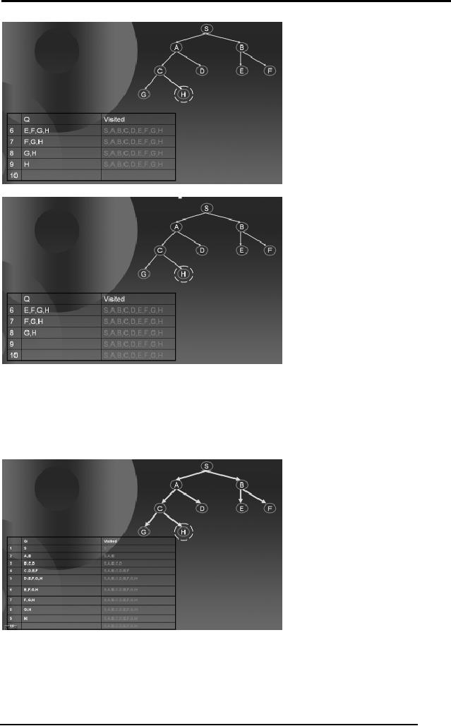
B and repeat. The following sequence of diagram tells you how the algorithm

proceeds till it reach the goal state.

Artificial Intelligence (CS607)

Artificial Intelligence (CS607)

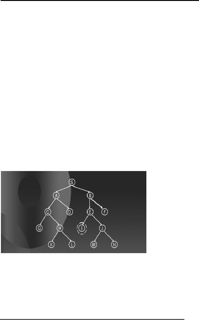
When we remove H from the 9th row of the table and check if it's the goal, the

algorithm says YES and hence we return H since we have reached the goal

state. The path followed by the BFS is shown by green arrows at each step. The

diagram below also shows that BFS travels a significant area of the search space

if the solution is located somewhere deep inside the tree.

Hence, simply by selecting a specific P(n) our Simple Search Algorithm was

converted to a BFS procedure.

Artificial Intelligence (CS607)

2.12 Problems with DFS and BFS

Though DFS and BFS are simple searching techniques which can get us to the

goal state very easily yet both of them have their own problems.

DFS has small space requirements (linear in depth) but has major problems:

DFS can run forever in search spaces with infinite length paths

DFS does not guarantee finding the shallowest goal

BFS guarantees finding the shallowest path even in presence of infinite paths,

but it has one great problem

BFS requires a great deal of space (exponential in depth)

We can still come up with a better technique which caters for the drawbacks of

both these techniques. One such technique is progressive deepening.

2.13 Progressive Deepening

Progressive deepening actually emulates BFS using DFS. The idea is to simply

apply DFS to a specific level. If you find the goal, exit, other wise repeat DFS to

the next lower level. Go on doing this until you either reach the goal node or the

full height of the tree is explored. For example, apply a DFS to level 2 in the tree,

if it reaches the goal state, exit, otherwise increase the level of DFS and apply it

again until you reach level 4. You can increase the level of DFS by any factor. An

example will further clarify your understanding.

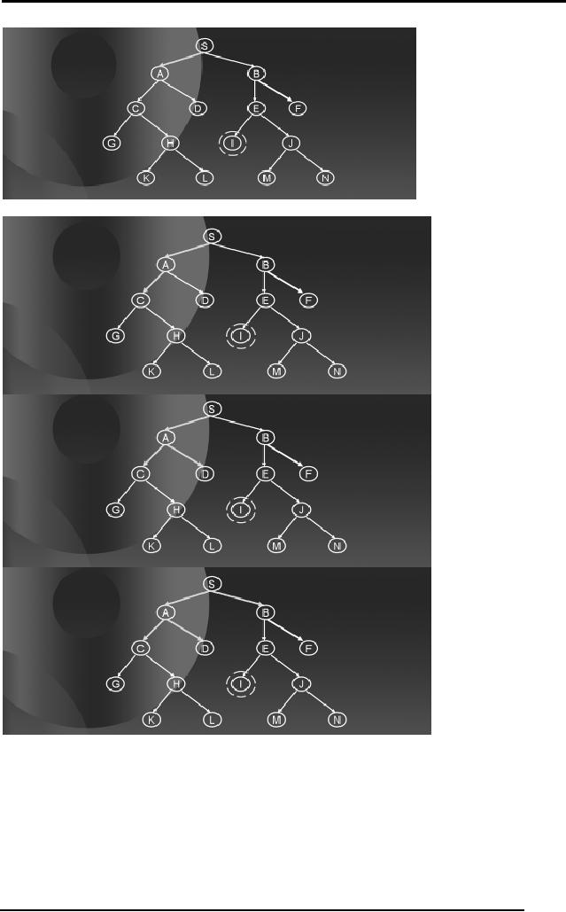
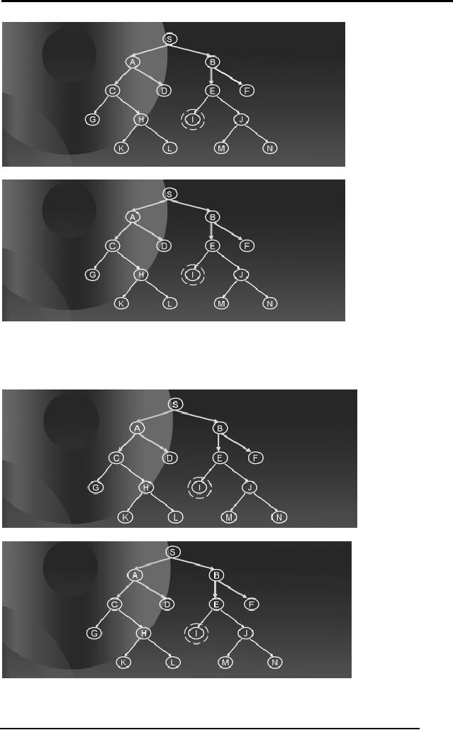
Consider the tree on the previous page with nodes from S ... to N, where I is the

goal node.

Apply DFS to level 2 in the tree. The green arrows in the diagrams below show

how DFS will proceed to level 2.

Artificial Intelligence (CS607)

Artificial Intelligence (CS607)

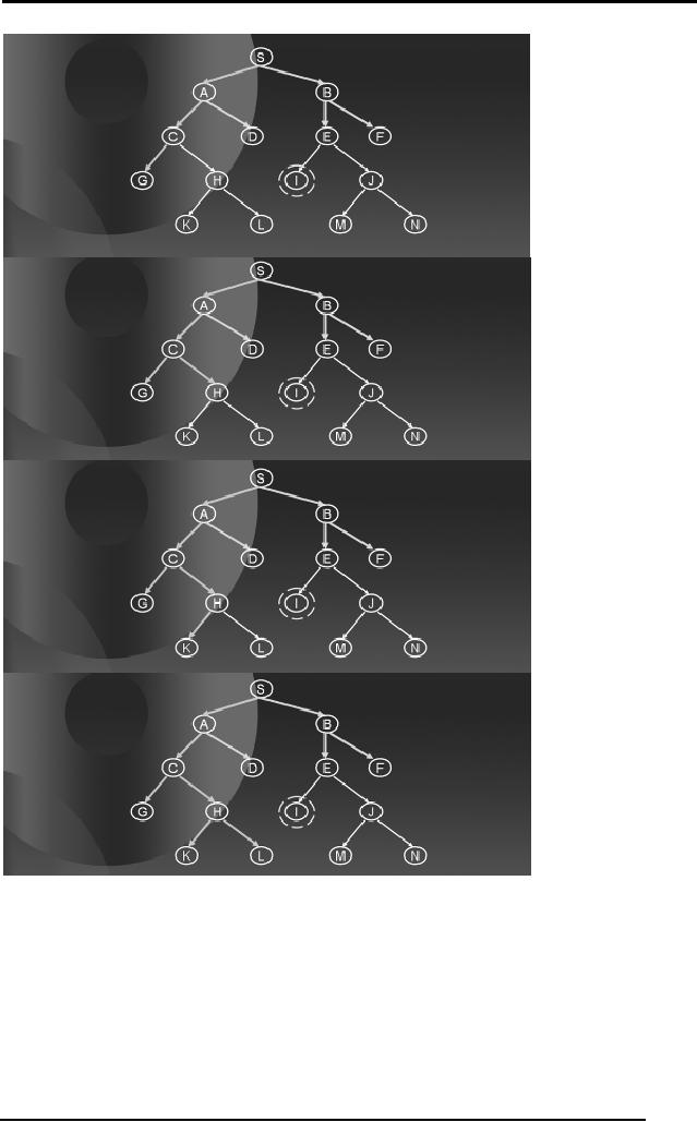
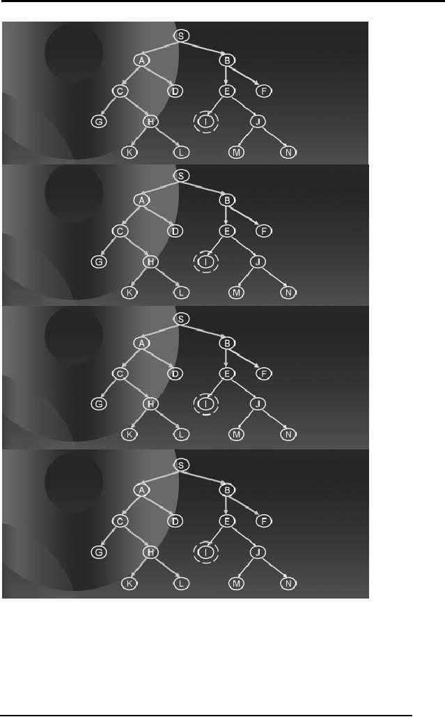
After exploring to level 2, the progressive deepening procedure will find out that

the goal state has still not been reached. Hence, it will increment the level by a

factor of, say 2, and will now perform a DFS in the tree to depth 4. The blue

arrows in the diagrams below show how DFS will proceed to level 4.

Artificial Intelligence (CS607)

Artificial Intelligence (CS607)

Artificial Intelligence (CS607)

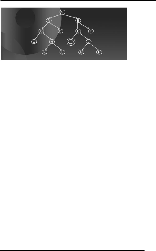
As soon as the procedure finds the goal state it will quit. Notice that it guarantees

to find the solution at a minimum depth like BFS. Imagine that there are a number

of solutions below level 4 in the tree. The procedure would only travel a small

portion of the search space and without large memory requirements, will find out

the solution.

2.14 Heuristically Informed Searches

So far we have looked into procedures that search the solution space in an

uninformed manner. Such procedures are usually costly with respect to either

time, space or both. We now focus on a few techniques that search the solution

space in an informed manner using something which is called a heuristic. Such

techniques are called heuristic searches. The basic idea of a heuristic search is

that rather than trying all possible search paths, you try and focus on paths that

seem to be getting you closer to your goal state using some kind of a "guide". Of

course, you generally can't be sure that you are really near your goal state.

However, we might be able to use a good guess for the purpose. Heuristics are

used to help us make that guess. It must be noted that heuristics don't always

give us the right guess, and hence the correct solutions. In other words educated

guesses are not always correct.

Recall the example of the mouse searching for cheese. The smell of cheese

guides the mouse in the maze, in other words the strength of the smell informs

the mouse that how far is it from the goal state. Here the smell of cheese is the

heuristic and it is quite accurate.

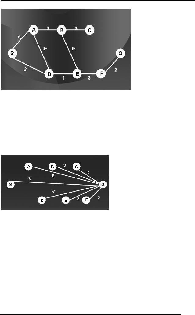
Similarly, consider the diagram below. The graph shows a map in which the

numbers on the edges are the distances between cities, for example, the

distance between city S and city D is 3 and between B and E is 4.

Artificial Intelligence (CS607)

Suppose our goal is to reach city G starting from S. There can be many choices,

we might take S, A, D, E, F, G or travel from S, to A, to E, to F, and to G. At each

city, if we were to decide which city to go next, we might be interested in some

sort of information which will guide us to travel to the city from which the distance

of goal is minimum.

If someone can tell us the straight-line distance of G from each city then it might

help us as a heuristic in order to decide our route map. Consider the graph

below.

It shows the straight line distances from every city to the goal. Now, cities that are

closer to the goal should be our preference. These straight line distances also

known as "as the crow flies distance" shall be our heuristic.

It is important to note that heuristics can sometimes misguide us. In the example

we have just discussed, one might try to reach city C as it is closest from the goal

according to our heuristic, but in the original map you can see that there is no

direct link between city C and city G. Even if someone reaches city C using the

heuristic, he won't be able to travel to G from C directly, hence the heuristic can

misguide. The catch here is that crow-flight distances do not tell us that the two

cities are directly connected.

Similarly, in the example of mouse and cheese, consider that the maze has

fences fixed along some of the paths through which the smell can pass. Our

heuristic might guide us on a path which is blocked by a fence, hence again the

heuristic is misguiding us.

Artificial Intelligence (CS607)

The conclusion then is that heuristics do help us reduce the search space, but it

is not at all guaranteed that we'll always find a solution. Still many people use

them as most of the time they are helpful. The key lies in the fact that how do we

use the heuristic. Consider the notion of a heuristic function.

Whenever we choose a heuristic, we come up with a heuristic function which

takes as input the heuristic and gives us out a number corresponding to that

heuristic. The search will now be guided by the output of the heuristic function.

Depending on our application we might give priority to either larger numbers or

smaller numbers.

Hence to every node/ state in our graph we will assign a heuristic value,

calculated by the heuristic function. We will start with a basic heuristically

informed search which is called Hill Climbing.

2.15 Hill Climbing

Hill Climbing is basically a depth first search with a measure of quality that is

assigned to each node in the tree. The basic idea is: Proceed as you would in

DFS except that you order your choices according to some heuristic

measurement of the remaining distance to the goal. We will discuss the Hill

climbing with an example.

Before going to the actual example, let us give another analogy for which the

name Hill Climbing has been given to this procedure. Consider a blind person

climbing a hill. He can not see the peak of the hill. The best he can do is that from

a given point he takes steps in all possible directions and wherever he finds that

a step takes him higher he takes that step and reaches a new, higher point. He

goes on doing this until all possible steps in any direction will take him higher and

this would be the peak, hence the name hill climbing. Notice that each step that

we take, gets us closer to our goal which in this example is the peak of a hill.

Such a procedure might as well have some problems.

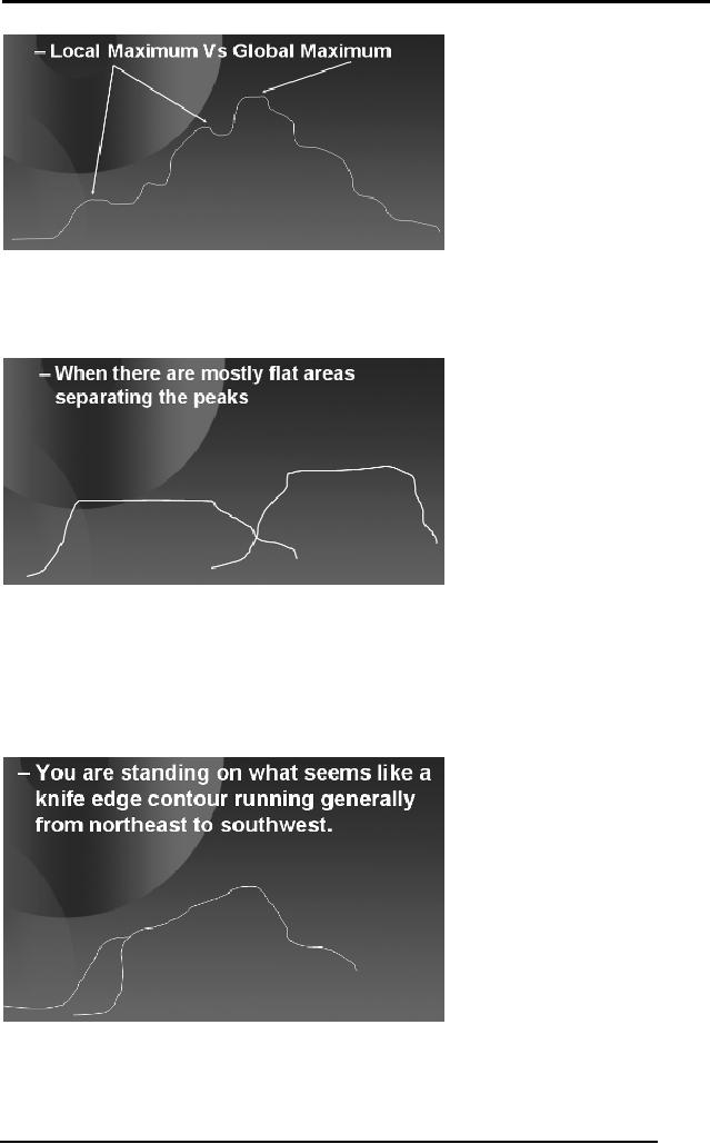
Foothill Problem: Consider the diagram of a mountain below. Before reaching

the global maxima, that is the highest peak, the blind man will encounter local

maxima that are the intermediate peaks and before reaching the maximum

height. At each of these local maxima, the blind man gets the perception of

having reached the global maxima as none of the steps takes him to a higher

point. Hence he might just reach local maxima and think that he has reached the

global maxima. Thus getting stuck in the middle of searching the solution space.

Artificial Intelligence (CS607)

Plateau Problem: Similarly, consider another problem as depicted in the

diagram below. Mountains where flat areas called plateaus are frequently

encountered the blind person might again get stuck.

When he reaches the portion of a mountain which is totally flat, whatever step he

takes gives him no improvement in height hence he gets stuck.

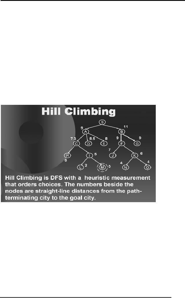
Ridge Problem: Consider another problem; you are standing on what seems like

a knife edge contour running generally from northeast to southwest. If you take

step in one direction it takes you lower, on the other hand when you step in some

other direction it gives you no improvement.

All these problems can be mapped to situations in our solution space searching.

If we are at a state and the heuristics of all the available options take us to a

lower value, we might be at local maxima. Similarly, if all the available heuristics

Artificial Intelligence (CS607)

take us to no improvement we might be at a plateau. Same is the case with ridge

as we can encounter such states in our search tree.

The solution to all these problems is randomness. Try taking random steps in

random direction of random length and you might get out of the place where you

are stuck.

Example

Let us now take you through an example of searching a tree using hill climbing to

end out discussion on hill climbing.

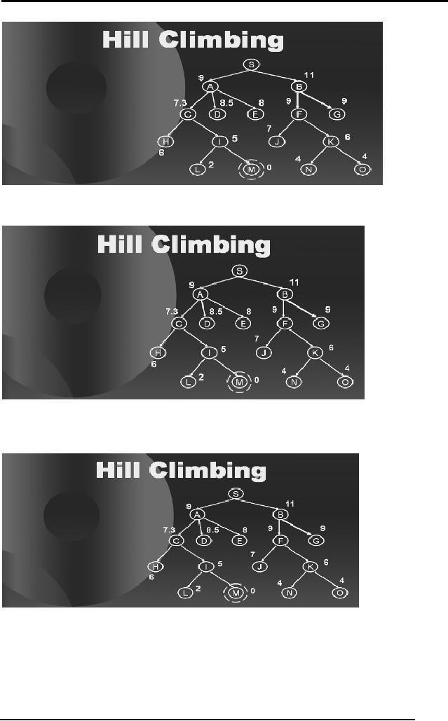
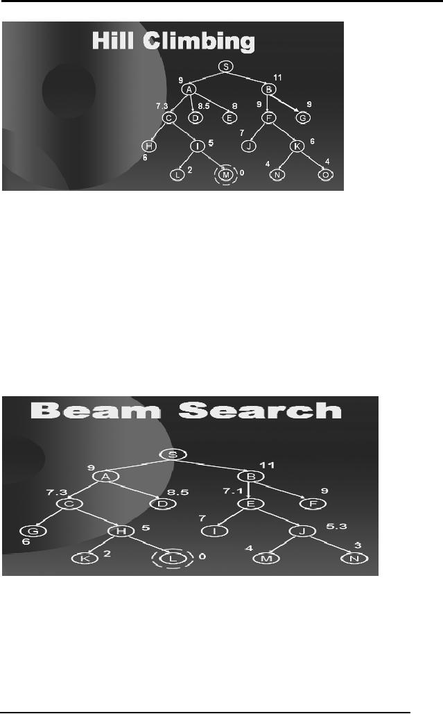
Consider the diagram below. The tree corresponds to our problem of reaching

city M starting from city S. In other words our aim is to find a path from S to M.

We now associate heuristics with every node, that is the straight line distance

from the path-terminating city to the goal city.

When we start at S we see that if we move to A we will be left with 9 units to

travel. As moving on A has given us an improvement in reaching our goal hence

we move to A. Exactly in the same manner as the blind man moves up a step

that gives him more height.

Artificial Intelligence (CS607)

Standing on A we see that C takes us closer to the goal hence we move to C.

From C we see that city I give us more improvement hence we move to I and

then finally to M.

Artificial Intelligence (CS607)

Notice that we only traveled a small portion of the search space and reached our

goal. Hence the informed nature of the search can help reduce space and time.

2.16 Beam Search

You just saw how hill climbing procedure works through the search space of a

tree. Another procedure called beam search proceeds in a similar manner. Out of

n possible choices at any level, beam search follows only the best k of them; k is

the parameter which we set and the procedure considers only those many nodes

at each level.

The following sequence of diagrams will show you how Beam Search works in a

search tree.

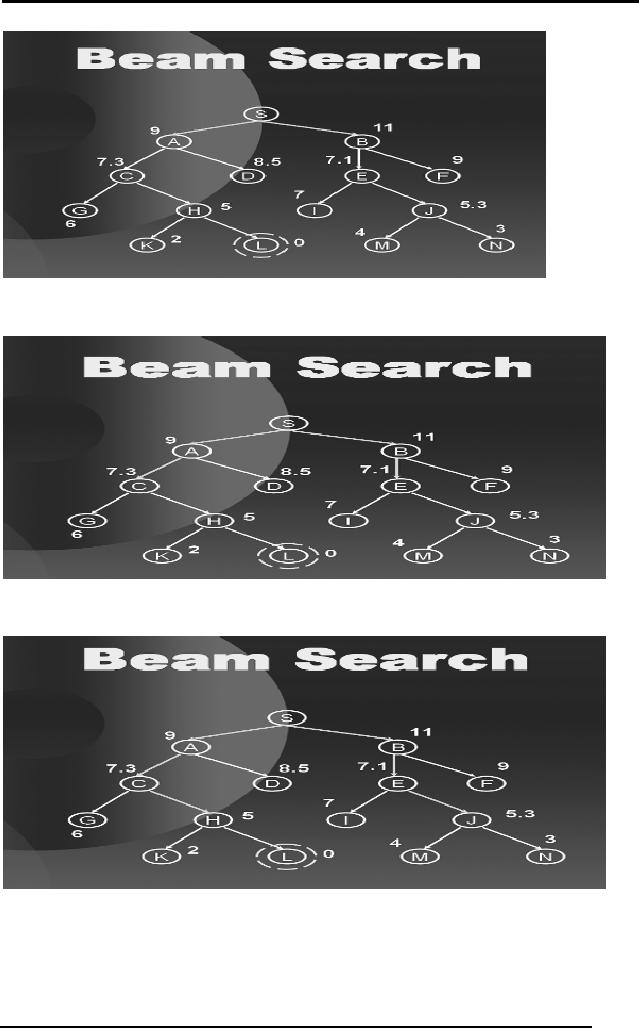
We start with a search tree with L as goal state and k=2, that is at every level we

will only consider the best 2 nodes. When standing on S we observe that the only

two nodes available are A and B so we explore both of them as shown below.

Artificial Intelligence (CS607)

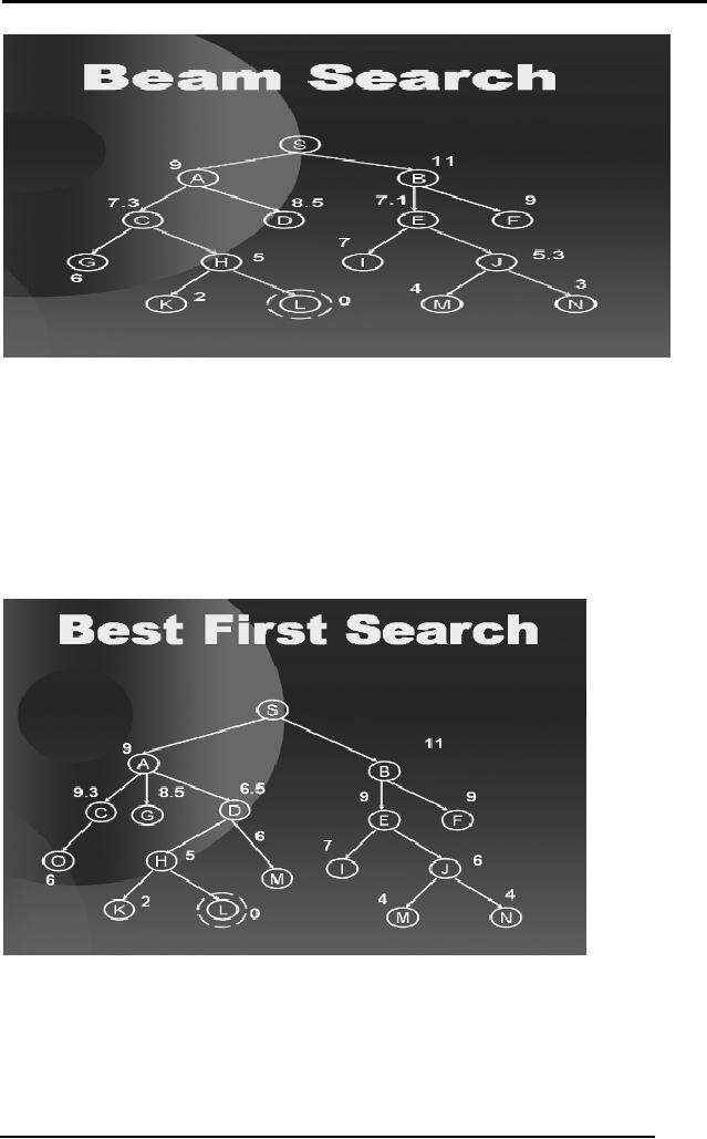
From here we have C, D, E and F as the available options to go. Again, we select

the two best of them and we explore C and E as shown in the diagram below.

From C and E we have G, H, I and J as the available options so we select H and

J and similarly at the last level we select L and N of which L is the goal.

Artificial Intelligence (CS607)

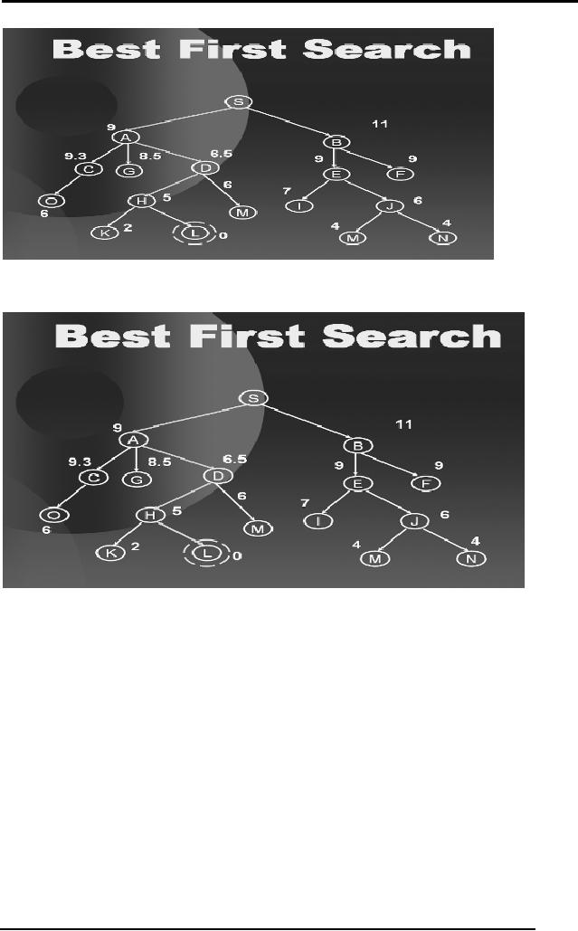
2.17 Best First Search

Just as beam search considers best k nodes at every level, best first search

considers all the open nodes so far and selects the best amongst them. The

following sequence of diagrams will show you how a best first search procedure

works in a search tree.

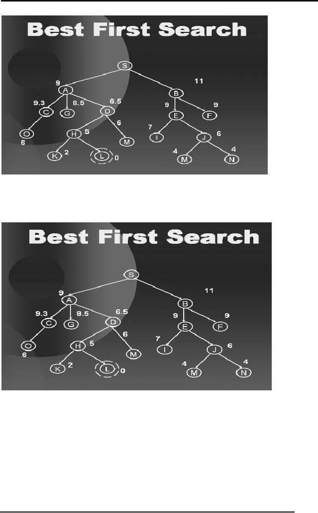
We start with a search tree as shown above. From S we observe that A is the

best option so we explore A.

Artificial Intelligence (CS607)

At A we now have C, G, D and B as the options. We select the best of them

which is D.

Artificial Intelligence (CS607)

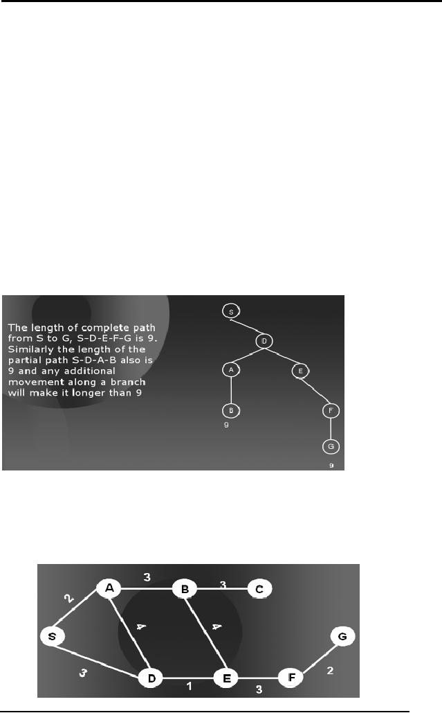
At D we have S, G, B, H, M and J as the options. We select H which is the best of

them.

At last from H we find L as the best. Hence best first search is a greedy approach

will looks for the best amongst the available options and hence can sometimes

reduce the searching time. All these heuristically informed procedures are

considered better but they do not guarantee the optimal solution, as they are

dependent on the quality of heuristic being used.

2.18 Optimal Searches

So far we have looked at uninformed and informed searches. Both have their

advantages and disadvantages. But one thing that lacks in both is that whenever

they find a solution they immediately stop. They never consider that their might

be more than one solution to the problem and the solution that they have ignored

might be the optimal one.

A simplest approach to find the optimal solution is this; find all the possible

solutions using either an uninformed search or informed search and once you

have searched the whole search space and no other solution exists, then choose

Artificial Intelligence (CS607)

the most optimal amongst the solutions found. This approach is analogous to the

brute force method and is also called the British museum procedure.

But in reality, exploring the entire search space is never feasible and at times is

not even possible, for instance, if we just consider the tree corresponding to a

game of chess (we will learn about game trees later), the effective branching

factor is 16 and the effective depth is 100. The number of branches in an

exhaustive survey would be on the order of 10120. Hence a huge amount of

computation power and time is required in solving the optimal search problems in

a brute force manner.

2.19 Branch and Bound

In order to solve our problem of optimal search without using a brute force

technique, people have come up with different procedures. One such procedure

is called branch-and-bound method.

The simple idea of branch and bound is the following:

The length of the complete path from S to G is 9. Also note that while traveling

from S to B we have already covered a distance of 9 units. So traveling further

from S D A B to some other node will make the path longer. So we ignore any

further paths ahead of the path S D A B.

We will show this with a simple example.

Artificial Intelligence (CS607)

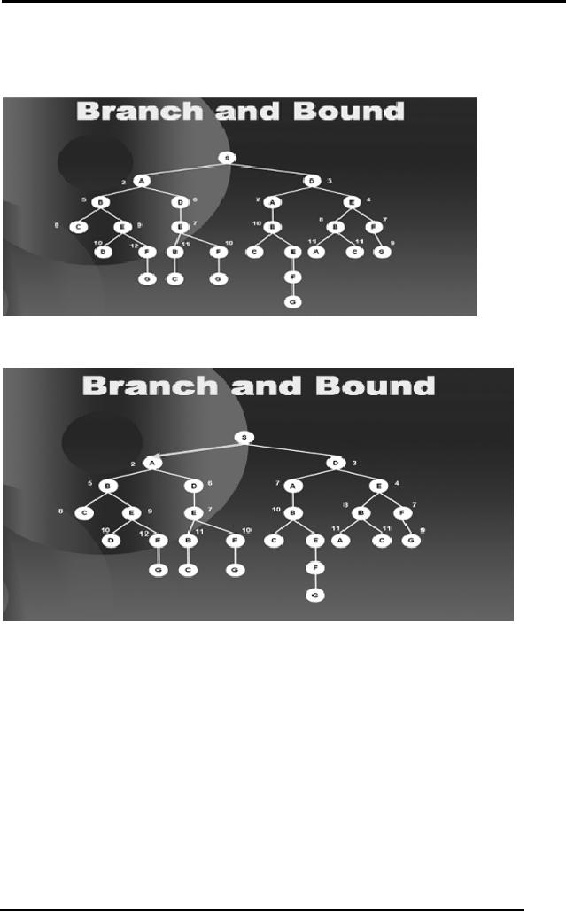
The diagram above shows the same city road map with distance between the

cities labels on the edges. We convert the map to a tree as shown below.

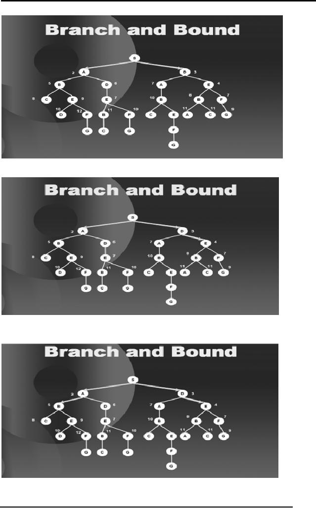
We proceed in a Best First Search manner. Starting at S we see that A is the

best option so we explore A.

From S the options to travel are B and D, the children of A and D the child of S.

Among these, D the child of S is the best option. So we explore D.

Artificial Intelligence (CS607)

From here the best option is E so we go there,

then B,

then D,

Artificial Intelligence (CS607)

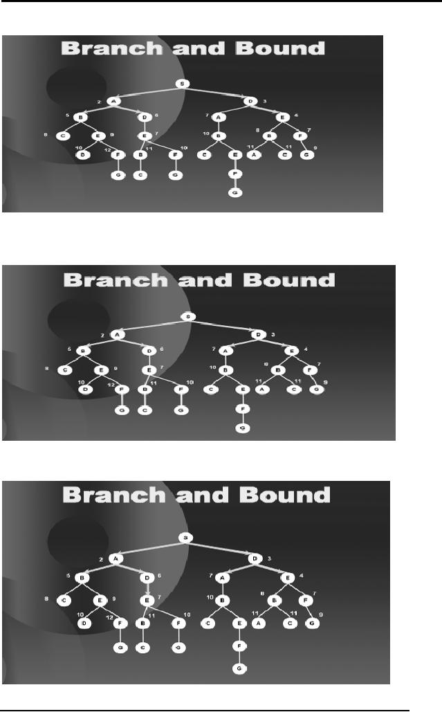
Here we have E, F and A as equally good options so we select arbitrarily and

move to say A,

then E.

Artificial Intelligence (CS607)

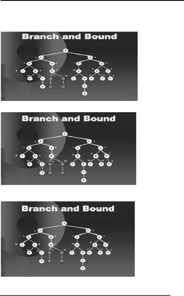
When we explore E we find out that if we follow this path further, our path length

will increase beyond 9 which is the distance of S to G. Hence we block all the

further sub-trees along this path, as shown in the diagram below.

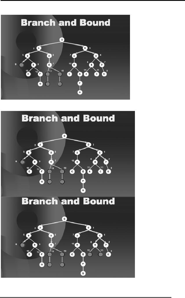
We then move to F as that is the best option at this point with a value 7.

then C,

We see that C is a leaf node so we bind C too as shown in the next diagram.

Artificial Intelligence (CS607)

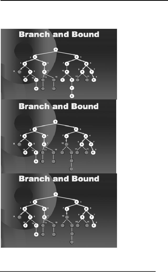
Then we move to B on the right hand side of the tree and bind the sub trees

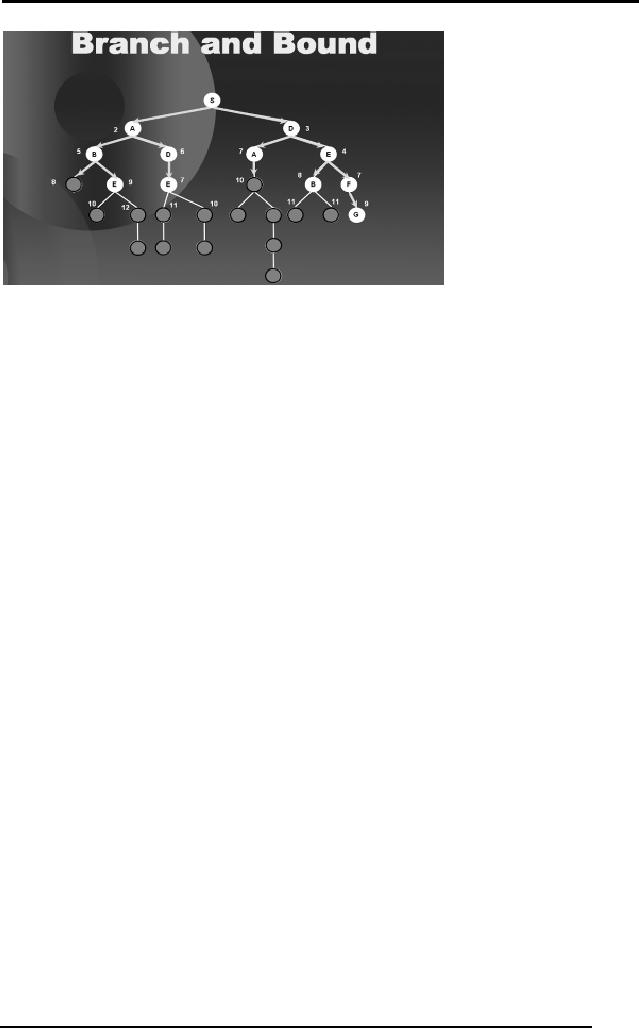
ahead of B as they also exceed the path length 9.

Artificial Intelligence (CS607)

We go on proceeding in this fashion, binding the paths that exceed 9 and hence

we are saved from traversing a considerable portion of the tree. The subsequent

diagrams complete the search until it has found all the optimal solution, that is

along the right hand branch of the tree.

Artificial Intelligence (CS607)

Notice that we have saved ourselves from traversing a considerable portion of

the tree and still have found the optimal solution. The basic idea was to reduce

the search space by binding the paths that exceed the path length from S to G.

2.20 Improvements in Branch and Bound

The above procedure can be improved in many different ways. We will discuss

the two most famous ways to improve it.

1. Estimates

2. Dynamic Programming

The idea of estimates is that we can travel in the solution space using a heuristic

estimate. By using "guesses" about remaining distance as well as facts about

distance already accumulated we will be able to travel in the solution space more

efficiently. Hence we use the estimates of the remaining distance. A problem

here is that if we go with an overestimate of the remaining distance then we might

loose a solution that is somewhere nearby. Hence we always travel with

underestimates of the remaining distance. We will demonstrate this improvement

with an example.

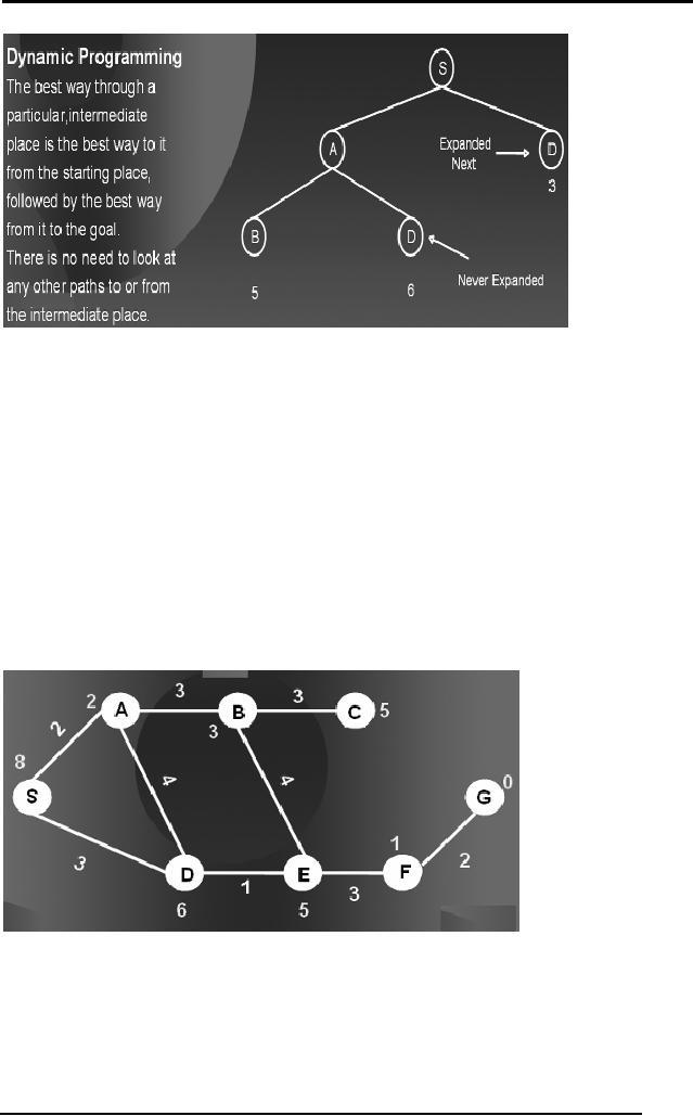
The second improvement is dynamic programming. The simple idea behind

dynamic programming is that if we can reach a specific node through more than

one different path then we shall take the path with the minimum cost.

Artificial Intelligence (CS607)

In the diagram you can see that we can reach node D directly from S with a cost

of 3 and via S A D with a cost of 6 hence we will never expand the path with the

larger cost of reaching the same node.

When we include these two improvements in branch and bound then we name it

as a different technique known as A* Procedure.

2.21 A* Procedure

This is actually branch and bound technique with the improvement of

underestimates and dynamic programming.

We will discuss the technique with the same example as that in branch-and-

bound.

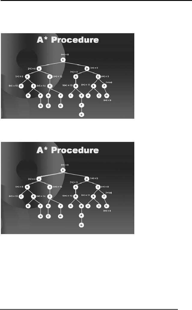
The values on the nodes shown in yellow are the underestimates of the distance

of a specific node from G. The values on the edges are the distance between two

adjacent cities.

Artificial Intelligence (CS607)

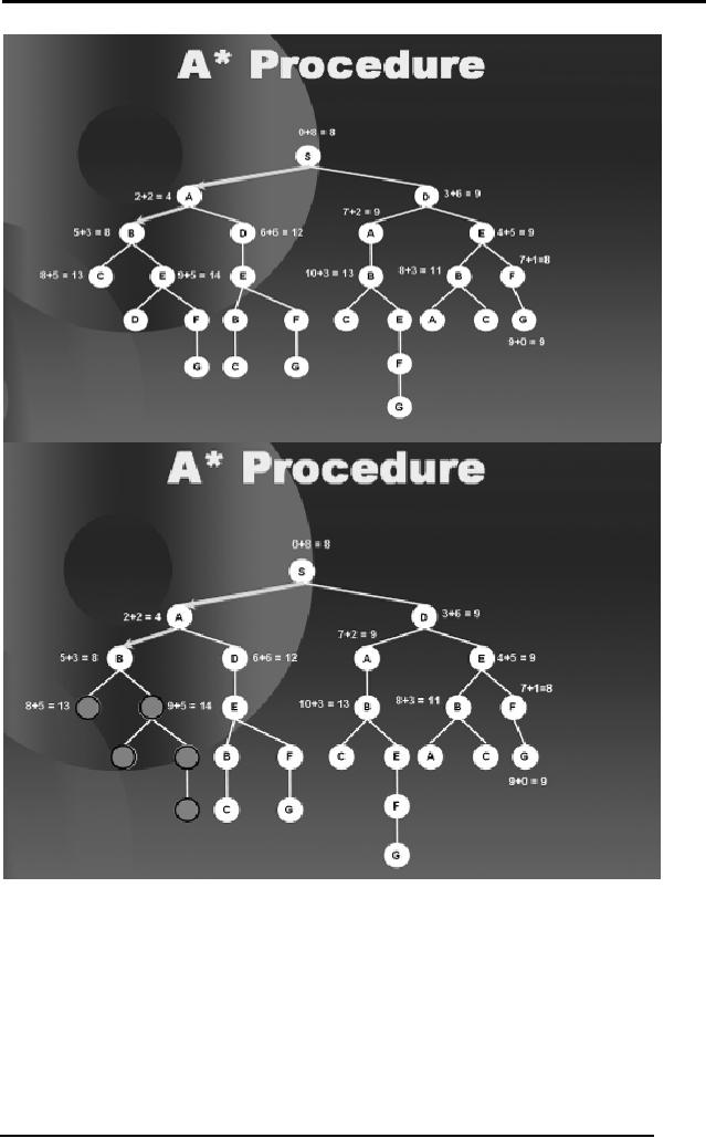
Our measure of goodness and badness of a node will now be decided by a

combination of values that is the distance traveled so far and the estimate of the

remaining distance. We construct the tree corresponding to the graph above.

We start with a tree with goodness of every node mentioned on it.

Standing at S we observe that the best node is A with a value of 4 so we move to

Then B. As all the sub-trees emerging from B make our path length more than 9

units so we bound this path, as shown in the next diagram.

Artificial Intelligence (CS607)

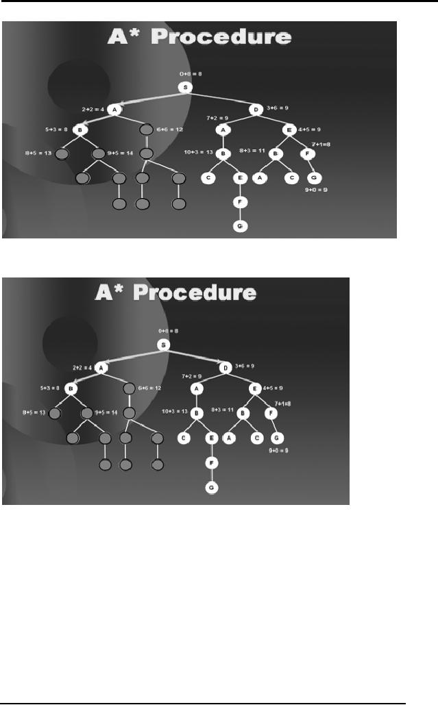
Now observe that to reach node D that is the child of A we can reach it either with

a cost of 12 or we can directly reach D from S with a cost of 9. Hence using

dynamic programming we will ignore the whole sub-tree beneath D (the child of

A) as shown in the next diagram.

Artificial Intelligence (CS607)

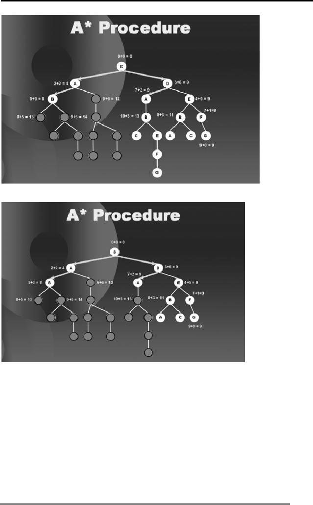
Now we move to D from S.

Now A and E are equally good nodes so we arbitrarily choose amongst them,

and we move to A.

Artificial Intelligence (CS607)

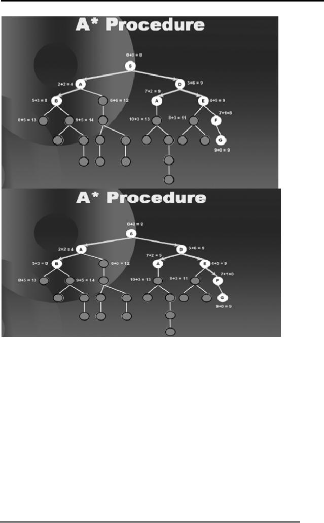
As the sub-tree beneath A expands the path length is beyond 9 so we bind it.

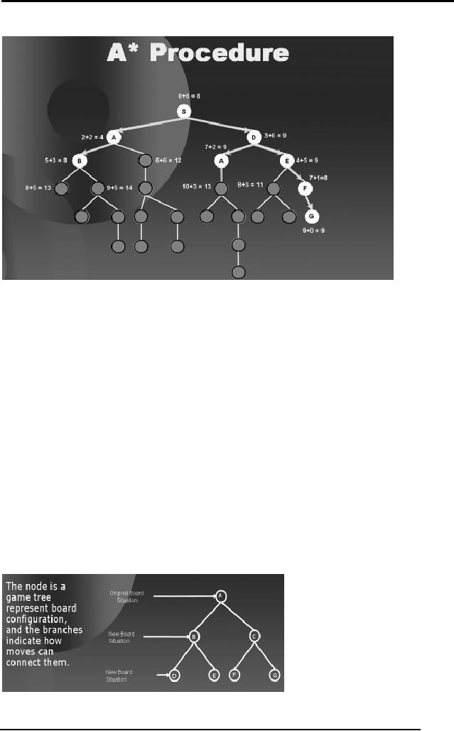
We proceed in this manner. Next we visit E, then we visit B the child of E, we

bound the sub-tree below B. We visit F and finally we reach G as shown in the

subsequent diagrams.

Artificial Intelligence (CS607)

Artificial Intelligence (CS607)

Notice that by using underestimates and dynamic programming the search space

was further reduced and our optimal solution was found efficiently.

2.22 Adversarial Search

Up until now all the searches that we have studied there was only one person or

agent searching the solution space to find the goal or the solution. In many

applications there might be multiple agents or persons searching for solutions in

the same solution space.

Such scenarios usually occur in game playing where two opponents also called

adversaries are searching for a goal. Their goals are usually contrary to each

other. For example, in a game of tic-tac-toe player one might want that he should

complete a line with crosses while at the same time player two wants to complete

a line of zeros. Hence both have different goals. Notice further that if player one

puts a cross in any box, player-two will intelligently try to make a move that would

leave player-one with minimum chance to win, that is, he will try to stop player-

one from completing a line of crosses and at the same time will try to complete

his line of zeros.

Many games can be modeled as trees as shown below. We will focus on board

games for simplicity.

Artificial Intelligence (CS607)

Searches in which two or more players with contrary goals are trying to explore

the same solution space in search of the solution are called adversarial searches.

2.23 Minimax Procedure

In adversarial searches one player tries to cater for the opponent's moves by

intelligently deciding that what will be the impact of his own move on the over all

configuration of the game. To develop this stance he uses a look ahead thinking

strategy. That is, before making a move he looks a few levels down the game

tree to see that what can be the impact of his move and what options will be open

to the opponent once he has made this move.

To clarify the concept of adversarial search let us discuss a procedure called the

minimax procedure.

Here we assume that we have a situation analyzer that converts all judgments

about board situations into a single, over all quality number. This situation

analyzer is also called a static evaluator and the score/ number calculated by the

evaluator is called the static evaluation of that node. Positive numbers, by

convention indicate favor to one player. Negative numbers indicate favor to the

other player. The player hoping for positive numbers is called maximizing player

or maximizer. The other player is called minimizing player or minimizer. The

maximizer has to keep in view that what choices will be available to the minimizer

on the next step. The minimizer has to keep in view that what choices will be

available to the maximizer on the next step.

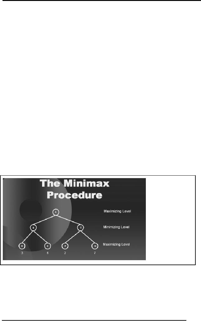
Consider the following diagram.

Artificial Intelligence (CS607)

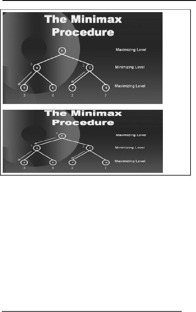
Standing at node A the maximizer wants to decide which node to visit next, that

is, choose between B or C. The maximizer wishes to maximize the score so

apparently 7 being the maximum score, the maximizer should go to C and then to

G. But when the maximizer will reach C the next turn to select the node will be of

the minimizer, which will force the game to reach configuration/node F with a

score of 2. Hence maximizer will end up with a score of 2 if he goes to C from A.

On the other hand, if the maximizer goes to B from A the worst which the

minimizer can do is that he will force the maximizer to a score of 3. Now, since

the choice is between scores of 3 or 2, the maximizer will go to node B from A.

2.24 Alpha Beta Pruning

In Minimax Procedure, it seems as if the static evaluator must be used on each

leaf node. Fortunately there is a procedure that reduces both the tree branches

that must be generated and the number of evaluations. This procedure is called

Alpha Beta pruning which "prunes" the tree branches thus reducing the number

of static evaluations.

We use the following example to explain the notion of Alpha Beta Pruning.

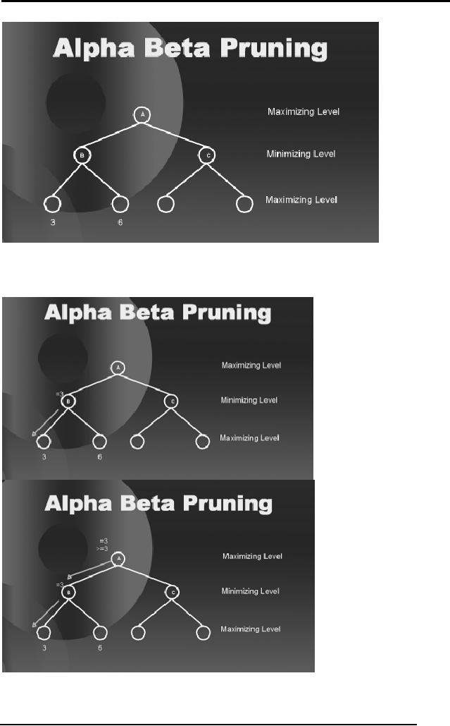
Suppose we start of with a game tree in the diagram below. Notice that all

nodes/situations have not yet been previously evaluated for their static evaluation

score. Only two leaf nodes have been evaluated so far.

Artificial Intelligence (CS607)

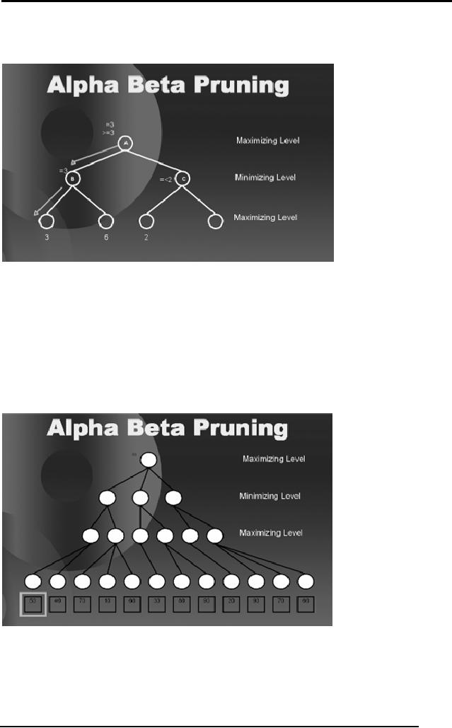
Sitting at A, the player-one will observe that if he moves to B the best he can get

is 3.

Artificial Intelligence (CS607)

So the value three travels to the root A. Now after observing the other side of the

tree, this score will either increase or will remain the same as this level is for the

maximizer.

When he evaluates the first leaf node on the other side of the tree, he will see

that the minimizer can force him to a score of less than 3 hence there is no need

to fully explore the tree from that side. Hence the right most branch of the tree will

be pruned and won't be evaluated for static evaluation.

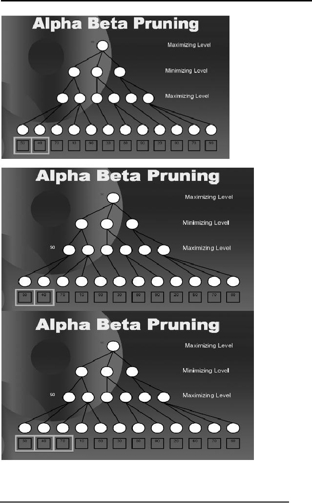
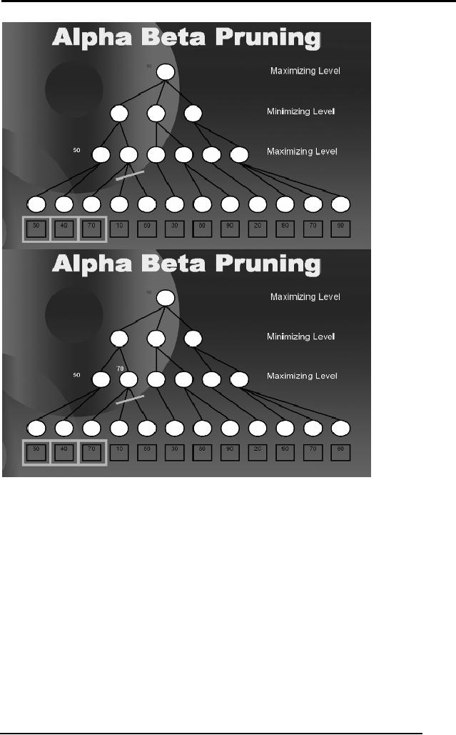
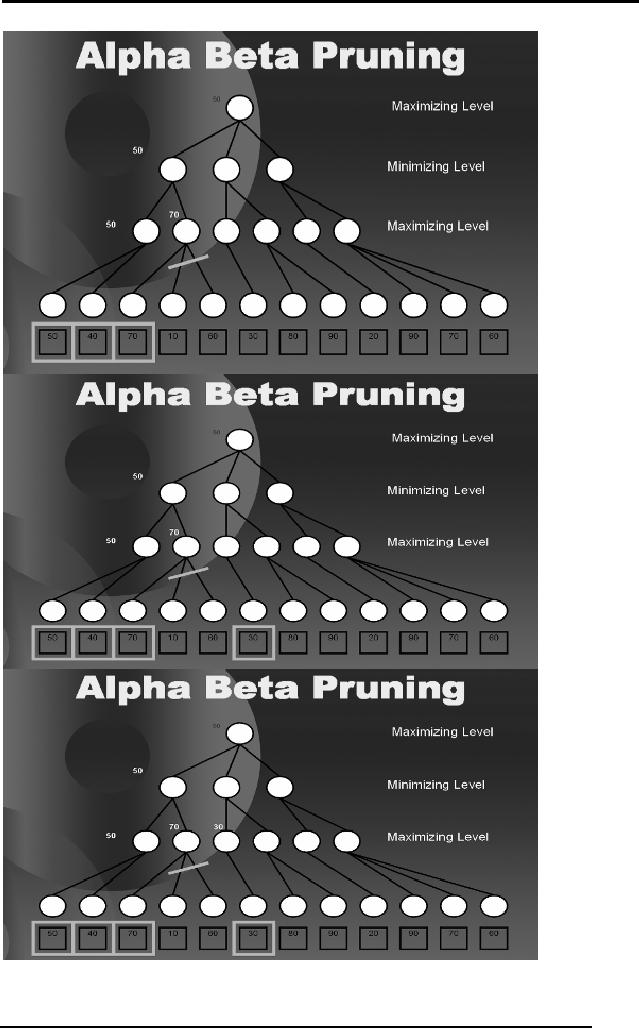
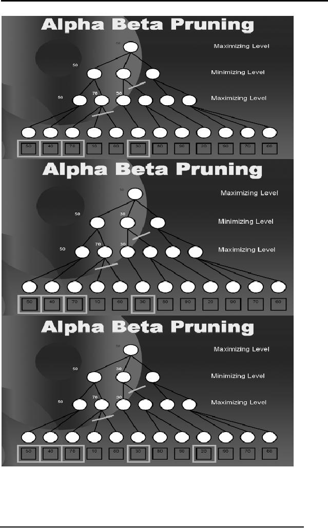
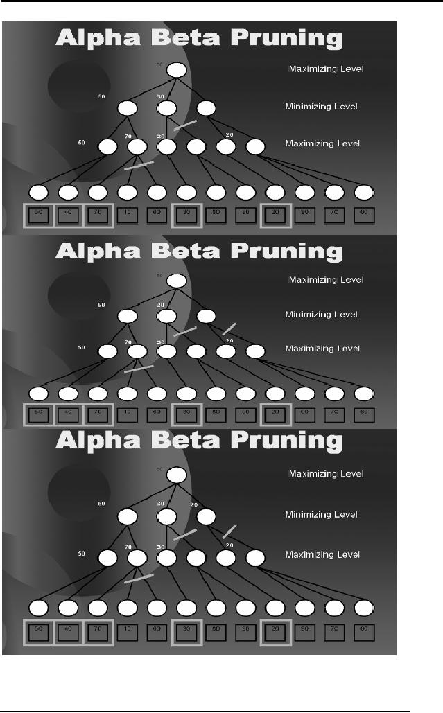
We have discussed a detailed example on Alpha Beta Pruning in the lectures.

We have shown the sequence of steps in the diagrams below. The readers are

required to go though the last portion of Lecture 10 for the explanation of this

example, if required.

Artificial Intelligence (CS607)

Artificial Intelligence (CS607)

Artificial Intelligence (CS607)

Artificial Intelligence (CS607)

Artificial Intelligence (CS607)

2.25 Summary

People used to think that one who can solve more problems is more intelligent

Artificial Intelligence (CS607)

Generate and test is the classical approach to solving problems

Problem representation plays a key role in problem solving

The components of problem solving include

o Problem Statement

o Operators

o Goal State

o Solution Space

Searching is a formal mechanism to explore alternatives

Searches can be blind or uninformed, informed, heuristic, non-optimal and

optional.

Different procedures to implement different search strategies form the major

content of this chapter

2.26 Problems

Q1 Consider that a person has never been to the city air port. Its early in the

morning and assume that no other person is awake in the town who can guide

him on the way. He has to drive on his car but doesn't know the way to air port.

Clearly identify the four components of problem solving in the above statement,

i.e. problem statement, operators, solution space, and goal state. Should he

follow blind or heuristic search strategy? Try to model the problem in a graphical

representation.

Q2 Clearly identify the difference between WSP (Well-Structured Problems) and

ISP (Ill- Structured) problems as discussed in the lecture. Give relevant

examples.

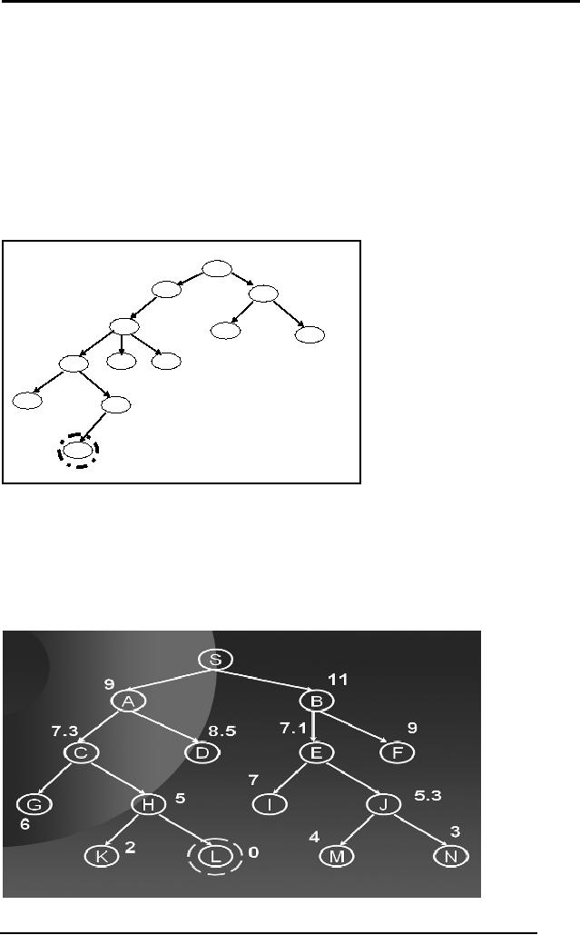
Q3 Given the following tree. Apply DFS and BFS as studied in the chapter. Show

the state of the data structure Q and the visited list clearly at every step. S is the

initial state and D is the goal state.

Artificial Intelligence (CS607)

Q4 Discuss how progressive deepening uses a mixture of DFS and BFS to

eliminate the disadvantages of both and at the same time finds the solution is a

given tree. Support your answer with examples of a few trees.

Q5 Discuss the problems in Hill Climbing. Suggest solutions to the commonly

encountered problems that are local maxima, plateau problem and ridge problem.

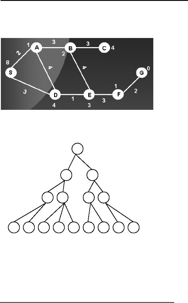
Given the following tree, use the hill climbing procedure to climb up the tree. Use

your suggested solutions to the above mention problems if any of them are

encountered. K is the goal state and numbers written on each node is the

estimate of remaining distance to the goal.

Q6 Discuss how best first search works in a tree. Support your answer with an

example tree. Is best first search always the best strategy? Will it always

guarantee the best solution?

Q7 Discuss how beam search with degree of the search = 3 propagates in the

given search tree. Is it equal to best first search when the degree = 1.

Artificial Intelligence (CS607)

Q8 Discuss the main concept behind branch and bound search strategy. Suggest

Improvements in the Algorithm. Simulate the algorithm on the given graph below.

The values on the links are the distances between the cities. The numbers on the

nodes are the estimated distance on the node from the goal state.

Q9. Run the MiniMax procedure on the given tree. The static evaluation scores

for each leaf node are written under it. For example the static evaluation scores

for the left most leaf node is 80.

100

Q10 Discuss how Alpha Beta Pruning minimizes the number of static evaluations

at the leaf nodes by pruning branches. Support your answer with small examples

of a few trees.

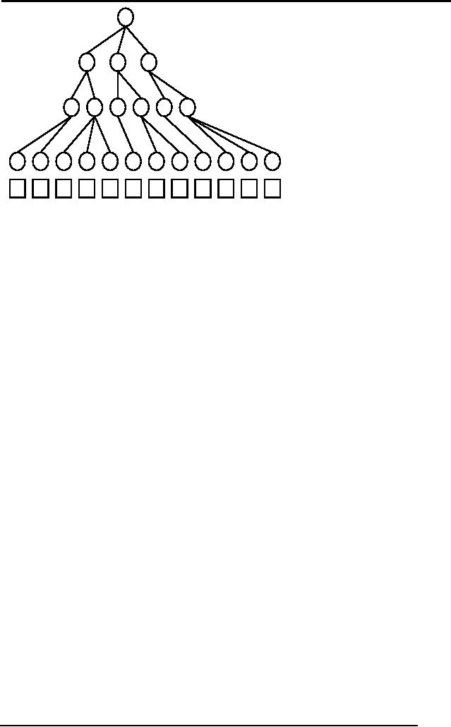
Q11 Simulate the Minimax procedure with Alpha Beta Pruning algorithm on the

following search tree.

Artificial Intelligence (CS607)

Maximizing Level

Minimizing Level

Maximizing Level

Adapted from: Artificial Intelligence, Third Edition by Patrick Henry Winston

Table of Contents: