 |

...Image
Processing Fundamentals
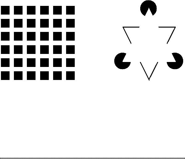
Figure
15: Optical
Illusions
The
left illusion induces the
illusion of gray values in
the eye that the
brain
"knows"
does not exist. Further,
there is a sense of dynamic
change in the image
due, in
part, to the saccadic movements of
the eye. The right
illusion, Kanizsa's
triangle,
shows enhanced contrast and
false contours [14] neither
of which can be
explained
by the system-oriented aspects of
visual perception described above.
5.
Image
Sampling
Converting
from a continuous image a(x,y)
to its digital representation b[m,n]
requires
the process of sampling. In
the ideal sampling system
a(x,y) is
multiplied
by
an ideal 2D impulse
train:
+∞
+∞
∑
∑δ (x - m Xo , y
- nYo )
=
a( x,
y
) �
bideal [ m.n]
m
=-∞
n
=-∞
(52)
+∞
+∞
∑
∑ a(
mXo , nYo )δ
(
x
- mX o, y
- nYo )
=
m=
- ∞ n=-∞
where
Xo and
Yo are
the sampling distances or
intervals and δ(�,�) is
the ideal
impulse
function. (At some point, of
course, the impulse function δ(x,y)
is
converted
to the discrete impulse
function δ[m,n].)
Square sampling
implies
that Xo
=Yo. Sampling
with an impulse function corresponds to
sampling with an
infinitesimally
small point. This, however,
does not correspond to the
usual
situation
as illustrated in Figure 1. To take the
effects of a finite
sampling
aperture
p(x,y)
into account, we can modify
the sampling model as
follows:
+∞
+∞
∑
∑ δ (
x
- m Xo , y
- nYo )
b[m.n
] =
( a(x, y)
⊗
p( x,
y))
�
(53)
m=-∞
n=-∞
28

...Image
Processing Fundamentals
The
combined effect of the aperture and
sampling are best understood
by
examining
the Fourier domain
representation.
+∞
+∞
1
∑
∑ A(Ω- mΩ s, Ψ
- nΨs
) � P (Ω
- mΩ s
, Ψ
- nΨs
)
B(Ω,
Ψ ) =
(54)
4� 2
m=-∞
n
=-∞
where
Ωs
= 2�/Xo is the
sampling frequency in the
x
direction and
Ψs
= 2�/Yo is
the
sampling frequency in the
y
direction.
The aperture p(x,y)
is frequently square,
circular,
or Gaussian with the associated
P
(Ω,Ψ). (See
Table 4.) The
periodic
nature
of the spectrum, described in
eq. (21) is clear from
eq. (54).
5.1
SAMPLING DENSITY FOR
IMAGE P
ROCESSING
To
prevent the possible aliasing
(overlapping) of
spectral terms that is
inherent in
eq.
(54) two conditions must
hold:
�
Bandlimited A(u,v)
A
(u,
v) ≡
0
u
> uc
v
> vc
for
and
(55)
�
Nyquist sampling frequency
Ω
s
> 2
� uc
and
Ψs
> 2
� vc
(56)
where
uc and
vc are the
cutoff
frequencies in the
x
and
y
direction,
respectively.
Images
that are acquired through
lenses that are circularly-symmetric,
aberration-
free,
and diffraction-limited will, in
general, be bandlimited. The
lens acts as a
lowpass
filter with a cutoff
frequency in the frequency
domain (eq. (11)) given
by:
2
NA
uc = v c =
(57)
λ
where
NA
is the
numerical aperture of the
lens and λ
is
the shortest wavelength
of
light
used with the lens [16]. If
the lens does not meet one
or more of these
assumptions
then it will still be bandlimited
but at lower cutoff
frequencies than
those
given in eq. (57). When
working with the F-number
(F
) of the
optics instead
of
the NA
and in
air (with index
of refraction = 1.0),
eq. (57) becomes:
2
1
uc = v c =
(58)
λ
4F2 +
1
29

...Image
Processing Fundamentals
5.1.1
Sampling aperture
The
aperture p
(x,y) described
above will have only a
marginal effect on the
final
signal
if the two conditions eqs.
(56) and (57) are satisfied.
Given, for example,
the
distance
between samples Xo equals Yo and a
sampling aperture that is
not wider
than
Xo, the
effect on the overall
spectrum--due to the A(u,v)P (u,v)
behavior
implied
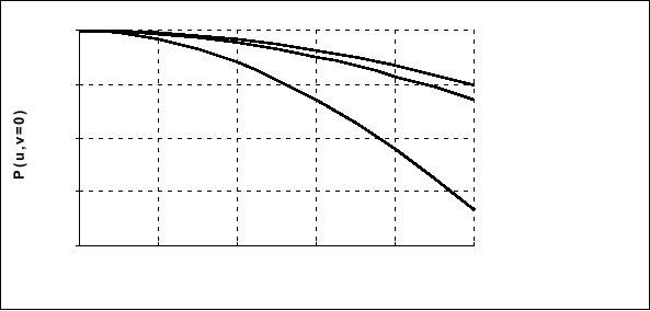
by eq.(53)--is illustrated in Figure 16
for square and Gaussian
apertures.
The
spectra are evaluated along
one axis of the 2D Fourier
transform. The Gaussian
aperture
in Figure 16 has a width
such that the sampling
interval Xo contains
�3σ
(99.7%)
of the Gaussian. The
rectangular apertures have a
width such that one
occupies
95% of the sampling interval
and the other occupies 50% of
the sampling
interval.
The 95% width translates to a
fill
factor of 90%
and the 50% width to a
fill
factor
of 25%.
The fill
factor is discussed in
Section 7.5.2.
1.0
--
Square aperture,
0.9
fill
= 25%
--
Gaussian
aperture
0.8
0.7
--
Square aperture,
fill
= 90%
0.6
0.0
0.1
0.2
0.3
0.4
0.5
Fraction
of Nyquist frequency
Figure
16: Aperture
spectra P
(u,v=0)
for frequencies up to half the
Nyquist
frequency.
For explanation of "fill"
see text.
5.2
SAMPLING DENSITY FOR
IMAGE ANALYSIS
The
"rules" for choosing the
sampling density when the
goal is image analysis--as
opposed
to image processing--are different. The
fundamental difference is that
the
digitization
of objects in an image into a
collection of pixels introduces a
form of
spatial
quantization noise that is not
bandlimited. This leads to
the following results
for
the choice of sampling
density when one is
interested in the measurement
of
area
and (perimeter)
length.
30

...Image
Processing Fundamentals
5.2.1
Sampling for area
measurements
Assuming
square sampling, Xo = Yo and the unbiased
algorithm for estimating
area
which
involves simple pixel
counting, the CV
(see
eq. (38)) of the
area
measurement
is related to the sampling density by
[17]:
lim
CV
( S)
=
k2S
- 3
2
lim
CV
(S
) =
k3S
- 2
2D :
3D :
(59)
S
→∞
S
→∞
and
in D
dimensions:
lim
CV
(S
) =
k
DS- (
D+1
) 2
(60)
S
→∞
where
S
is the
number of samples per
object diameter. In 2D the
measurement is
area,
in 3D volume, and in D-dimensions
hypervolume.
5.2.2
Sampling for length
measurements
Again
assuming square sampling and
algorithms for estimating
length based upon
the
Freeman chain-code representation
(see Section 3.6.1), the
CV
of the
length
measurement
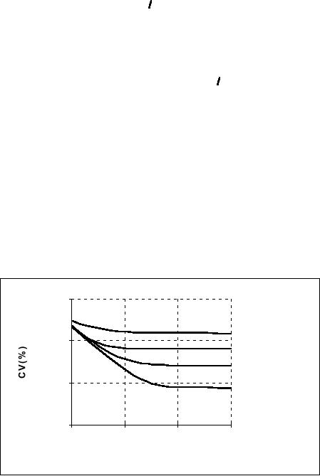
is related to the sampling
density per
unit length as shown in
Figure
17
(see [18, 19].)
100.0%
Pixel
Count
10.0%
Freeman
Kulpa
1.0%
Corner
Count
0.1%
1
10
100
1000
Sampling
Density / Unit Length
Figure
17: CV
of length
measurement for various
algorithms.
The
curves in Figure 17 were
developed in the context of
straight lines but
similar
results
have been found for
curves and closed contours.
The specific formulas
for
length
estimation use a chain code
representation of a line and
are based upon a
linear
combination of three
numbers:
L
= α �
Ne + β �
No + γ �
Nc
(61)
31
Table of Contents:
- Introduction
- Digital Image Definitions:COMMON VALUES, Types of operations, VIDEO PARAMETERS
- Tools:CONVOLUTION, FOURIER TRANSFORMS, Circularly symmetric signals
- Perception:BRIGHTNESS SENSITIVITY, Wavelength sensitivity, OPTICAL ILLUSIONS
- Image Sampling:Sampling aperture, Sampling for area measurements
- Noise:PHOTON NOISE, THERMAL NOISE, KTC NOISE, QUANTIZATION NOISE
- Cameras:LINEARITY, Absolute sensitivity, Relative sensitivity, PIXEL FORM
- Displays:REFRESH RATE, INTERLACING, RESOLUTION
- Algorithms:HISTOGRAM-BASED OPERATIONS, Equalization, Binary operations, Second Derivatives
- Techniques:SHADING CORRECTION, Estimate of shading, Unsharp masking
- Acknowledgments
- References