Tools:CONVOLUTION, FOURIER TRANSFORMS, Circularly symmetric signals

<< Digital Image Definitions:COMMON VALUES, Types of operations, VIDEO PARAMETERS

Perception:BRIGHTNESS SENSITIVITY, Wavelength sensitivity, OPTICAL ILLUSIONS >>

...Image Processing Fundamentals

Standard

NTSC

PAL

SECAM

Property

images / second

29.97

ms / image

33.37

40.0

lines / image

525

625

(horiz./vert.) = aspect ratio

4:3

interlace

2:1

µs / line

63.56

64.00

Table 3: Standard video parameters

In an interlaced image the odd numbered lines (1,3,5,...) are scanned in half of the

allotted time (e.g. 20 ms in PAL) and the even numbered lines (2,4,6,...) are

scanned in the remaining half. The image display must be coordinated with this

scanning format. (See Section 8.2.) The reason for interlacing the scan lines of a

video image is to reduce the perception of flicker in a displayed image. If one is

planning to use images that have been scanned from an interlaced video source, it is

important to know if the two half-images have been appropriately "shuffled" by the

digitization hardware or if that should be implemented in software. Further, the

analysis of moving objects requires special care with interlaced video to avoid

"zigzag" edges.

The number of rows (N) from a video source generally corresponds onetoone

with lines in the video image. The number of columns, however, depends on the

nature of the electronics that is used to digitize the image. Different frame grabbers

for the same video camera might produce M = 384, 512, or 768 columns (pixels)

per line.

Tools

Certain tools are central to the processing of digital images. These include

mathematical tools such as convolution, Fourier analysis, and statistical

descriptions, and manipulative tools such as chain codes and run codes. We will

present these tools without any specific motivation. The motivation will follow in

later sections.

3.1 CONVOLUTION

There are several possible notations to indicate the convolution of two (multi-

dimensional) signals to produce an output signal. The most common are:

c =a ⊗b = a∗b

(1)

...Image Processing Fundamentals

We shall use the first form, c = a ⊗ b , with the following formal definitions.

In 2D continuous space:

+∞ +∞

∫ ∫ a( χ ,ζ )b( x - χ , y - ζ )dχdζ

c (x, y) = a( x, y ) ⊗ b( x, y ) =

(2)

-∞ -∞

In 2D discrete space:

+∞

∑ ∑a[ j , k ]b[ m - j, n - k]

c[m, n] = a[m , n] ⊗ b[m, n] =

(3)

j=-∞ k =-∞

3.2 P ROPERTIES OF CONVOLUTION

There are a number of important mathematical properties associated with

convolution.

· Convolution is commutative.

c =a ⊗b = b⊗ a

(4)

· Convolution is associative.

c = a ⊗ (b ⊗ d ) = (a ⊗ b) ⊗ d = a ⊗ b ⊗ d

(5)

· Convolution is distributive.

c = a ⊗ (b + d ) = (a ⊗ b) + ( a ⊗ d)

(6)

where a, b, c, and d are all images, either continuous or discrete.

3.3 F OURIER TRANSFORMS

The Fourier transform produces another representation of a signal, specifically a

representation as a weighted sum of complex exponentials. Because of Euler's

formula:

e jq = cos(q ) + jsin( q)

(7)

where j 2 = -1 , we can say that the Fourier transform produces a representation of

a (2D) signal as a weighted sum of sines and cosines. The defining formulas for

the forward Fourier and the inverse Fourier transforms are as follows. Given an

image a and its Fourier transform A, then the forward transform goes from the

...Image Processing Fundamentals

spatial domain (either continuous or discrete) to the frequency domain which is

always continuous.

A = F {a}

(8)

Forward

The inverse Fourier transform goes from the frequency domain back to the spatial

domain.

a = F -1 {A}

(9)

Inverse

The Fourier transform is a unique and invertible operation so that:

{F -1 {A}}

{F {a}}

a = F -1

A= F

and

(10)

The specific formulas for transforming back and forth between the spatial domain

and the frequency domain are given below.

In 2D continuous space:

+∞ +∞

a (x, y)e - j(ux + vy) dxdy

∫

A(u, v) =

(11)

Forward

-∞ -∞

+∞ +∞

A(u, v)e + j (ux +vy )dudv

4š 2 -∫ -∫

a( x , y) =

(12)

Inverse

∞ ∞

In 2D discrete space:

+∞

∑ ∑a[ m, n ]e- j (Ωm +Ψn )

A(Ω, Ψ ) =

(13)

Forward

m =-∞ n=-∞

+ š +š

A(Ω, Ψ )e + j(Ωm +Ψn) dΩdΨ

∫

a[m, n] =

(14)

Inverse

4š 2

-š -š

3.4 P ROPERTIES OF F OURIER TRANSFORMS

There are a variety of properties associated with the Fourier transform and the

inverse Fourier transform. The following are some of the most relevant for digital

image processing.

...Image Processing Fundamentals

· The Fourier transform is, in general, a complex function of the real frequency

variables. As such the transform can be written in terms of its magnitude and

phase.

A(u, v) = A( u, v ) e jϕ (u, v)

A(Ω, Ψ) = A(Ω, Ψ) e jϕ ( Ω,Ψ)

(15)

· A 2D signal can also be complex and thus written in terms of its magnitude and

phase.

a( x , y) = a( x, y ) e jϑ( x, y)

a[m , n] = a[m, n] e jϑ[ m, n]

(16)

· If a 2D signal is real, then the Fourier transform has certain symmetries.

A(u, v) = A* ( -u, - v)

A(Ω, Ψ) = A* (-Ω, -Ψ )

(17)

The symbol (*) indicates complex conjugation. For real signals eq. (17) leads

directly to:

A(u, v) = A (- u, -v)

ϕ (u, v) = -ϕ ( -u, - v )

(18)

A(Ω, Ψ) = A(-Ω, -Ψ )

ϕ (Ω, Ψ) = -ϕ ( -Ω, -Ψ )

· If a 2D signal is real and even, then the Fourier transform is real and even.

A(u, v) = A(- u, -v )

A(Ω, Ψ ) = A(-Ω, -Ψ )

(19)

· The Fourier and the inverse Fourier transforms are linear operations.

F {w1a + w2 b} = F {w1 a} + F {w2 b} = w1 A + w2 B

(20)

F -1 {w1 A + w2B} = F -1 {w1 A} + F -1{w2 B} = w1 a + w2 b

where a and b are 2D signals (images) and w1 and w2 are arbitrary, complex

constants.

· The Fourier transform in discrete space, A(Ω,Ψ), is periodic in both Ω and Ψ.

Both periods are 2š.

A(Ω+ 2šj , Ψ + 2šk ) = A( Ω, Ψ)

j, k integers

(21)

· The energy, E , in a signal can be measured either in the spatial domain or the

frequency domain. For a signal with finite energy:

...Image Processing Fundamentals

Parseval's theorem (2D continuous space):

+∞ +∞

E = ∫ ∫ a( x, y) dxdy = 2

∫∫

A(u, v) 2 dudv

(22)

4š

-∞ -∞

Parseval's theorem (2D discrete space):

+š +š

+∞

E = ∑ ∑ a[m, n] = 2

∫∫

A(Ω, Ψ ) 2 dΩdΨ

(23)

4š

m=-∞ n=-∞

-š -š

This "signal energy" is not to be confused with the physical energy in the

phenomenon that produced the signal. If, for example, the value a[m,n] represents a

photon count, then the physical energy is proportional to the amplitude, a, and not

the square of the amplitude. This is generally the case in video imaging.

· Given three, multi-dimensional signals a, b, and c and their Fourier transforms A,

B , and C:

c =a ⊗b

↔

C = A· B

and

(24)

c =a· b

↔

2 A⊗B

4š

In words, convolution in the spatial domain is equivalent to multiplication in the

Fourier (frequency) domain and vice-versa. This is a central result which provides

not only a methodology for the implementation of a convolution but also insight

into how two signals interact with each other--under convolution--to produce a

third signal. We shall make extensive use of this result later.

· If a two-dimensional signal a(x,y) is scaled in its spatial coordinates then:

(

)

→

a( x, y )

a Mx · x , My · y

(25)





→

A u M , v M  M x · My

Then

A(u, v)



y

· If a two-dimensional signal a(x,y) has Fourier spectrum A(u,v) then:

+∞ +∞

∫ ∫ a( x, y )dxdy

A(u = 0, v = 0) =

-∞ -∞

(26)

+∞ +∞

2 ∫ ∫ A(u, v)dxdy

a( x = 0, y = 0 ) =

4š -∞ -∞

...Image Processing Fundamentals

· If a two-dimensional signal a(x,y) has Fourier spectrum A(u,v) then:

a( x, y) F

a(x , y) F

↔ juA(u, v)

↔ jvA(u, v)

(27)

a (x , y) F

a( x , y) F

↔ - u 2 A(u, v)

↔ - v 2 A(u, v)

3.4.1 Importance of phase and magnitude

Equation (15) indicates that the Fourier transform of an image can be complex.

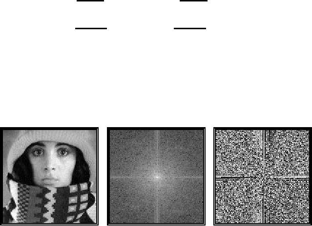
This is illustrated below in Figures 4a-c. Figure 4a shows the original image

a[m,n], Figure 4b the magnitude in a scaled form as log(|A(Ω,Ψ)|), and Figure 4c

the phase ϕ(Ω,Ψ).

Figure 4a

Figure 4b

Figure 4c

log(|A(Ω,Ψ)|)

ϕ(Ω,Ψ)

Original

Both the magnitude and the phase functions are necessary for the complete

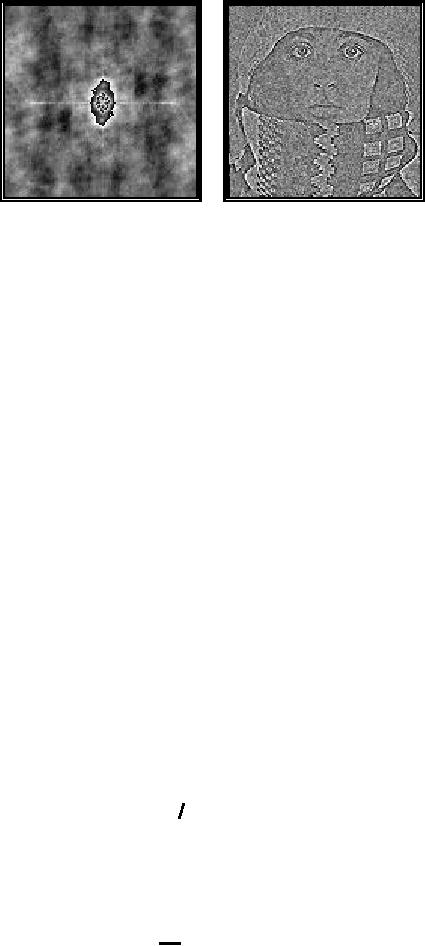
reconstruction of an image from its Fourier transform. Figure 5a shows what

happens when Figure 4a is restored solely on the basis of the magnitude

information and Figure 5b shows what happens when Figure 4a is restored solely

on the basis of the phase information.

...Image Processing Fundamentals

Figure 5a

Figure 5b

ϕ(Ω,Ψ) = 0

|A(Ω,Ψ)| = constant

Neither the magnitude information nor the phase information is sufficient to restore

the image. The magnitudeonly image (Figure 5a) is unrecognizable and has severe

dynamic range problems. The phase-only image (Figure 5b) is barely recognizable,

that is, severely degraded in quality.

3.4.2 Circularly symmetric signals

An arbitrary 2D signal a(x,y) can always be written in a polar coordinate system as

a(r,θ). When the 2D signal exhibits a circular symmetry this means that:

a( x , y) = a(r,θ ) = a(r )

(28)

where r2 = x2 + y2 and tanθ = y/x. As a number of physical systems such as lenses

exhibit circular symmetry, it is useful to be able to compute an appropriate Fourier

representation.

The Fourier transform A(u, v) can be written in polar coordinates A(ωr,ξ) and then,

for a circularly symmetric signal, rewritten as a Hankel transform:

∞

A(u, v) = F {a( x , y )} = 2š ∫ a(r )J o(ωr r)rdr = A (ω r )

(29)

where ω2 = u 2 + v 2 and tanξ = v u and Jo(·) is a Bessel function of the first kind

of order zero.

The inverse Hankel transform is given by:

∞

∫ A(ωr )J o(ω rr )ω rdω r

a( r) =

(30)

2š

...Image Processing Fundamentals

The Fourier transform of a circularly symmetric 2D signal is a function of only the

radial frequency, ωr. The dependence on the angular frequency, ξ, has vanished.

Further, if a(x,y) = a(r) is real, then it is automatically even due to the circular

symmetry. According to equation (19), A(ωr) will then be real and even.

3.4.3 Examples of 2D signals and transforms

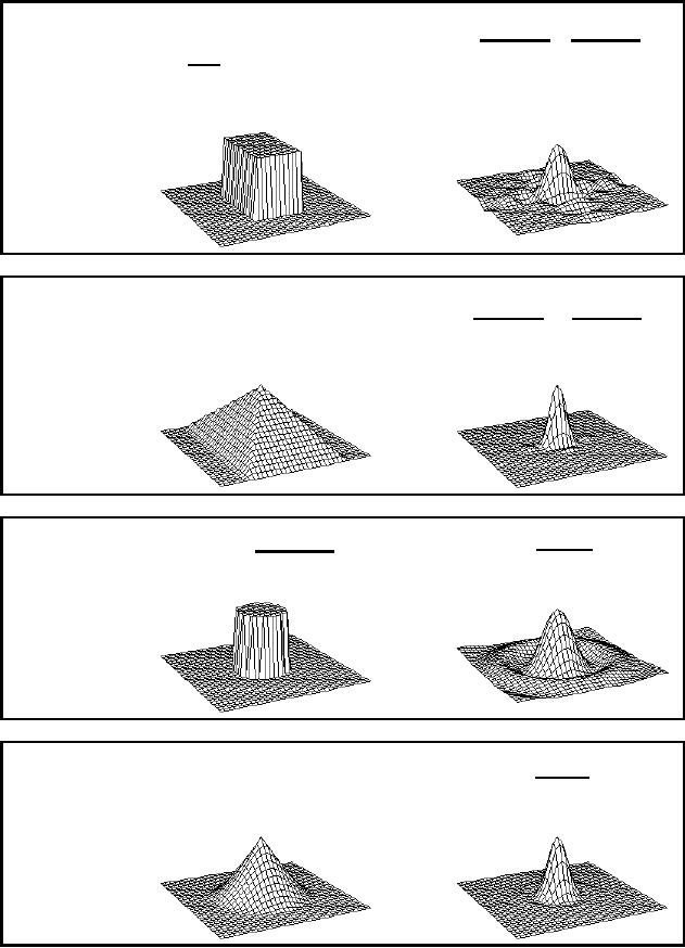
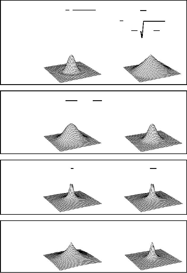
Table 4 shows some basic and useful signals and their 2D Fourier transforms. In

using the table entries in the remainder of this chapter we will refer to a spatial

domain term as the point spread function (PSF) or the 2D impulse response and its

Fourier transforms as the optical transfer function (OTF) or simply transfer

function. Two standard signals used in this table are u(·), the unit step function, and

J1(·), the Bessel function of the first kind. Circularly symmetric signals are treated

as functions of r as in eq. (28).

3.5 STATISTICS

In image processing it is quite common to use simple statistical descriptions of

images and subimages. The notion of a statistic is intimately connected to the

concept of a probability distribution, generally the distribution of signal amplitudes.

For a given region--which could conceivably be an entire image--we can define

the probability distribution function of the brightnesses in that region and the

probability density function of the brightnesses in that region. We will assume in

the discussion that follows that we are dealing with a digitized image a[m,n].

3.5.1 Probability distribution function of the brightnesses

The probability distribution function, P (a), is the probability that a brightness

chosen from the region is less than or equal to a given brightness value a. As a

increases from ∞ to + ∞, P (a) increases from 0 to 1. P (a) is monotonic, non-

decreasing in a and thus dP /da ≥ 0.

3.5.2 Probability density function of the brightnesses

The probability that a brightness in a region falls between a and a+Ća, given the

probability distribution function P (a), can be expressed as p(a)Ća where p(a) is the

probability density function:

 dP( a) 

p( a)Ć a = 

 Ća

(31)

 da 

...Image Processing Fundamentals

Ra, b ( x , y) =

 sin(aω x )   sin( bωy )

T.1 Rectangle

↔







 aω x   bω y 

u(a2 - x 2)u( b2 - y 2 )

4ab

Ra, b ( x , y) ⊗ Ra,b (x , y)

 sin(aω x )   sin( bω y )

T.2 Pyramid

↔



 



 aω x   bω y 

J1(aω ) 

u(a2 - r2 )

2

T.3 Cylinder

Pa (r ) =

↔



aω 

ša2

Pa (r ) ⊗ Pa(r )

J ( aω ) 

4 1

T.4 Cone

↔

 aω 

...Image Processing Fundamentals

1  J1(ω cr / 2 ) 2

 -1 ω 



T.5 Airy PSF

PSF(r ) = 

↔

cos   -







ωc 

2



u(ω c2 - ω

šω

2

ω 



  ω  1- ω  

 

  



G2 D( f , σ ) = exp(-ω 2σ 2 / 2)

 r2 

T.6 Gaussian

g2 D (r ,σ ) =

2 exp -

↔



 2σ 2 

2šσ

2š

T.7 Peak

↔

e - ar

2ša / (ω 2 + a 2 )3 / 2

T.8 Exponential

↔

Decay

Table 4: 2D Images and their Fourier Transforms

...Image Processing Fundamentals

Because of the monotonic, non-decreasing character of P (a) we have that:

+∞

∫ p(a)da = 1

p( a) ≥ 0

and

(32)

∞

For an image with quantized (integer) brightness amplitudes, the interpretation of

Ća is the width of a brightness interval. We assume constant width intervals. The

brightness probability density function is frequently estimated by counting the

number of times that each brightness occurs in the region to generate a histogram,

h[a]. The histogram can then be normalized so that the total area under the

histogram is 1 (eq. (32)). Said another way, the p[a] for a region is the normalized

count of the number of pixels, Λ, in a region that have quantized brightness a:

Λ = ∑ h[ a]

p[a] =

h[a]

with

(33)

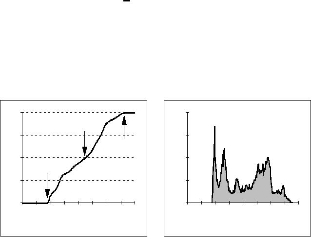
The brightness probability distribution function for the image shown in Figure 4a is

shown in Figure 6a. The (unnormalized) brightness histogram of Figure 4a which

is proportional to the estimated brightness probability density function is shown in

Figure 6b. The height in this histogram corresponds to the number of pixels with a

given brightness.

1.00

1600

median

0.75

1200

maximum

0.50

800

mimimum

0.25

400

0.00

64 96 128 160 192 224 256

32 64 96 128 160 192 224 256

Brightness

(a)

(b)

Figure 6: (a) Brightness distribution function of Figure 4a with minimum, median, and

maximum indicated. See text for explanation. (b) Brightness histogram of Figure 4a.

Both the distribution function and the histogram as measured from a region are a

statistical description of that region. It must be emphasized that both P [a] and p[a]

should be viewed as estimates of true distributions when they are computed from a

specific region. That is, we view an image and a specific region as one realization of

...Image Processing Fundamentals

the various random processes involved in the formation of that image and that

region. In the same context, the statistics defined below must be viewed as

estimates of the underlying parameters.

3.5.3 Average

The average brightness of a region is defined as the sample mean of the pixel

brightnesses within that region. The average, ma, of the brightnesses over the Λ

pixels within a region (ℜ) is given by:

∑ a[ m, n ]

ma =

(34)

Λ ( m, n)∈ℜ

Alternatively, we can use a formulation based upon the (unnormalized) brightness

histogram, h(a) = Λ·p(a), with discrete brightness values a. This gives:

∑ a · h[a]

ma =

(35)

Λ a

The average brightness, ma, is an estimate of the mean brightness, µa, of the

underlying brightness probability distribution.

3.5.4 Standard deviation

The unbiased estimate of the standard deviation, sa, of the brightnesses within a

region (ℜ) with Λ pixels is called the sample standard deviation and is given by:

∑ (a[ m, n] - ma )

Λ - 1 m,n ∈ℜ

(36)

∑ a2 [m, n] - Λma

m, n∈ℜ

Λ -1

Using the histogram formulation gives:





 ∑ a · h[a ] -Λ · ma

 a



(37)

Λ -1

The standard deviation, sa, is an estimate of σa of the underlying brightness

probability distribution.

...Image Processing Fundamentals

3.5.5 Coefficient-of-variation

The dimensionless coefficientofvariation, CV, is defined as:

CV =

× 100%

(38)

3.5.6 Percentiles

The percentile, p%, of an unquantized brightness distribution is defined as that

value of the brightness a such that:

P (a) = p%

or equivalently

∫ p(α )dα = p%

(39)

∞

Three special cases are frequently used in digital image processing.

the minimum value in the region

· 0%

the median value in the region

· 50%

the maximum value in the region

· 100%

All three of these values can be determined from Figure 6a.

3.5.7 Mode

The mode of the distribution is the most frequent brightness value. There is no

guarantee that a mode exists or that it is unique.

3.5.8 SignaltoNoise ratio

The signaltonoise ratio, SNR, can have several definitions. The noise is

characterized by its standard deviation, sn. The characterization of the signal can

differ. If the signal is known to lie between two boundaries, amin ≤ a ≤ amax, then

the SNR is defined as:

a

- amin 

SNR = 20 log10  max

 dB

(40)

Bounded signal





If the signal is not bounded but has a statistical distribution then two other

definitions are known:

Stochastic signal

 ma 

SNR = 20 log10   dB

(41)

S & N inter-dependent

 sn 

...Image Processing Fundamentals

s 

SNR = 20 log10  a  dB

(42)

S & N independent

 sn 

where ma and sa are defined above.

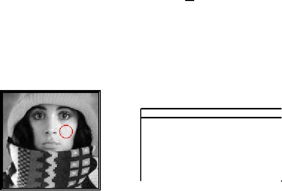
The various statistics are given in Table 5 for the image and the region shown in

Figure 7.

Statistic

Image

ROI

Average

137.7

219.3

Standard Deviation

49.5

4.0

Minimum

202

Median

141

220

Maximum

241

226

Mode

220

SNR (db)

33.3

Figure 7

Table 5

Region is the interior of the circle.

Statistics from Figure 7

A SNR calculation for the entire image based on eq. (40) is not directly available.

The variations in the image brightnesses that lead to the large value of s (=49.5) are

not, in general, due to noise but to the variation in local information. With the help

of the region there is a way to estimate the SNR. We can use the sℜ (=4.0) and the

dynamic range, amax amin, for the image (=24156) to calculate a global SNR

(=33.3 dB). The underlying assumptions are that 1) the signal is approximately

constant in that region and the variation in the region is therefore due to noise, and,

2) that the noise is the same over the entire image with a standard deviation given

by sn = sℜ.

3.6 CONTOUR REPRESENTATIONS

When dealing with a region or object, several compact representations are available

that can facilitate manipulation of and measurements on the object. In each case we

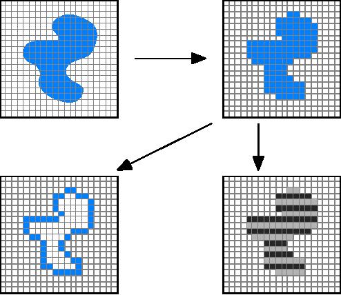
assume that we begin with an image representation of the object as shown in Figure

8a,b. Several techniques exist to represent the region or object by describing its

contour.

3.6.1 Chain code

This representation is based upon the work of Freeman [11]. We follow the

contour in a clockwise manner and keep track of the directions as we go from one

contour pixel to the next. For the standard implementation of the chain code we

...Image Processing Fundamentals

consider a contour pixel to be an object pixel that has a background (non-object)

pixel as one or more of its 4-connected neighbors. See Figures 3a and 8c.

The codes associated with eight possible directions are the chain codes and, with x

as the current contour pixel position, the codes are generally defined as:

321

Chain codes =

4 x 0

(43)

567

Digitization

(b)

(a)

Contour

Run Lengths

(c)

(d)

Figure 8: Region (shaded) as it is transformed from (a) continuous to (b)

discrete form and then considered as a (c) contour or (d) run lengths

illustrated in alternating colors.

3.6.2 Chain code properties

· Even codes {0,2,4,6} correspond to horizontal and vertical directions; odd codes

{1,3,5,7} correspond to the diagonal directions.

· Each code can be considered as the angular direction, in multiples of 45°, that we

must move to go from one contour pixel to the next.

· The absolute coordinates [m,n] of the first contour pixel (e.g. top, leftmost)

together with the chain code of the contour represent a complete description of the

discrete region contour.

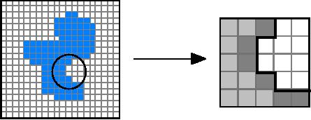
...Image Processing Fundamentals

· When there is a change between two consecutive chain codes, then the contour

has changed direction. This point is defined as a corner.

3.6.3 "Crack" code

An alternative to the chain code for contour encoding is to use neither the contour

pixels associated with the object nor the contour pixels associated with background

but rather the line, the "crack", in between. This is illustrated with an enlargement

of a portion of Figure 8 in Figure 9.

The "crack" code can be viewed as a chain code with four possible directions

instead of eight.

Crack codes = 2 x 0

(44)

Close up

(a)

(b)

Figure 9: (a) Object including part to be studied. (b) Conto ur

pixels as used in the chain code are diagonally shaded. The

"crack" is shown with the thick black line.

The chain code for the enlarged section of Figure 9b, from top to bottom, is

{5,6,7,7,0}. The crack code is {3,2,3,3,0,3,0,0}.

3.6.4 Run codes

A third representation is based on coding the consecutive pixels along a row--a

run--that belong to an object by giving the starting position of the run and the

ending position of the run. Such runs are illustrated in Figure 8d. There are a

number of alternatives for the precise definition of the positions. Which alternative

should be used depends upon the application and thus will not be discussed here.

Table of Contents: