AGGREGATE SUPPLY (Continued…):Deriving the Phillips Curve from SRAS

<< AGGREGATE SUPPLY:The sticky-price model

GOVERNMENT DEBT:Permanent Debt, Floating Debt, Unfunded Debts >>

Macroeconomics ECO 403

LESSON 34

AGGREGATE SUPPLY (Continued...)

Three Models of Aggregate Supply

Each of the three models of aggregate supply imply the relationship summarized by the SRAS

curve & equation

LRAS

Y = Y + α( - P )

> Pe

SRAS

<P e

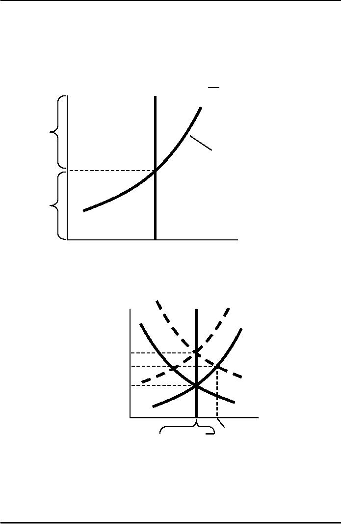
Suppose a positive AD shock moves output above its natural rate and P above the level people

had expected. Over time, P e rises, SRAS shifts up, and output returns to its natural rate.

SRAS2

LRAS

SRAS1

P3 = P

AD2

P 2 = P 1 = P1

AD1

=Y 1 =

Inflation, Unemployment, and the Phillips Curve

The Phillips curve states that š depends on

Expected inflation, še

158

Macroeconomics ECO 403

Cyclical unemployment: the deviation of the actual rate of unemployment from the

natural rate

Supply shocks, ν

š = š e - β (u - u n ) + ν

Where β > 0 is an exogenous constant.

Deriving the Phillips Curve from SRAS

The Philips curve in its modern form states that the inflation rate depends on three forces:

·Expected inflation.

·The deviation of unemployment from the natural rate, called cyclical unemployment.

·Supply shocks.

We can drive the Philips curve from our equation for aggregate supply.

Y = Y + α (P - P e )

(1)

According to aggregate supply equation:

P = P e + ( 1 α ) (Y -Y )

(2)

Here are the three steps. First, add to the right-hand side of the equation a supply shock v to

represent exogenous events (such as change in world's oil prices) that alter the price level and

shift the short run aggregate supply curve:

P = P e + ( 1 α ) (Y -Y ) + ν

(3)

Next, to go from the price level to inflation rates, subtract last year's price level P -1

from

both sides of equation to obtain

(P - P-1 ) = ( P e - P-1 ) + (1 α ) (Y -Y ) + ν

(4)

The term on the left hand side is the difference between current price level and last years price

level, which is inflation. The term on the right hand side is the difference between the expected

price level and last years price level, which is expected inflation. Therefore,

š = š e + ( 1 α ) (Y -Y ) + ν

(5)

Now to go from output to unemployment, recall Okun's law which gives a relationship between

two variables. We can write this as

(1 α ) (Y -Y ) = - β (u - u n )

(6)

Using this Okun's law relationship, we can substitute left-hand side value in equation number

5, and we obtain

š = š - β (u - u ) + ν

(7)

The Phillips Curve and SRAS

Y = Y + α (P - P e )

SRAS:

š = š e - β (u - u n ) + ν

Phillips curve:

SRAS curve:

output is related to unexpected movements in the price level

159

Macroeconomics ECO 403

Phillips curve:

unemployment is related to unexpected movements in the inflation rate

Adaptive expectations

Adaptive expectations: an approach that assumes people form their expectations of future

inflation based on recently observed inflation.

A simple example:

Expected inflation = last year's actual inflation

š e = š -1

Then, theP.C.becomes

š = š -1 - β (u - u ) + ν

Inflation inertia

In this form, the Phillips curve implies that inflation has inertia:

In the absence of supply shocks or cyclical unemployment, inflation will continue

indefinitely at its current rate.

Past inflation influences expectations of current inflation, which in turn influences the

wages & prices that people set.

Two causes of rising & falling inflation

Cost-push inflation: inflation resulting from supply shocks. Adverse supply shocks typically

raise production costs and induce firms to raise prices, "pushing" inflation up.

Demand-pull inflation: inflation resulting from demand shocks. Positive shocks to aggregate

demand cause unemployment to fall below its natural rate, which "pulls" the inflation rate

up.

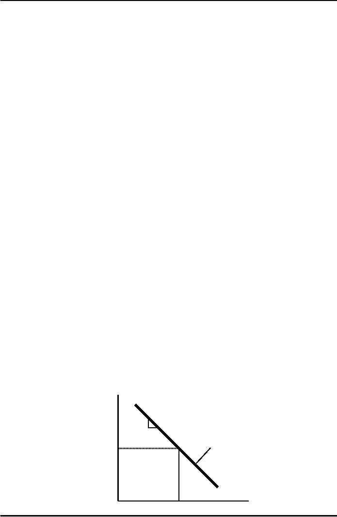
Graphing the Phillips curve

In the short run, policymakers face a trade-off between š and u.

The short-run Phillips

Curve

160

Macroeconomics ECO 403

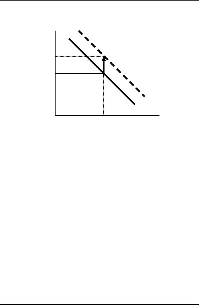
Shifting the Phillips curve

People adjust their expectations over time, so the tradeoff only holds in the short run. e.g., an

increase in še shifts the short-run P.C. upward.

š e +ν

š1 +ν

The sacrifice ratio

To reduce inflation, policymakers can

contract aggregate demand, causing

unemployment to rise above the natural rate.

The sacrifice ratio measures the percentage of a year's real GDP that must be foregone to

reduce inflation by 1 percentage point.

Estimates vary, but a typical one is 5.

Suppose policymakers wish to reduce inflation from 6 to 2 percent. If the sacrifice ratio is 5,

then reducing inflation by 4 points requires a loss of 4×5 = 20 percent of one year's GDP.

This could be achieved several ways, e.g.

Reduce GDP by 20% for one year

Reduce GDP by 10% for each of two years

Reduce GDP by 5% for each of four years

The cost of disinflation is lost GDP. One could use Okun's law to translate this cost into

unemployment.

Rational expectations

Ways of modeling the formation of expectations:

Adaptive expectations:

People base their expectations of future inflation on recently observed inflation.

Rational expectations:

People base their expectations on all available information, including information about

current a& prospective future policies.

161

Macroeconomics ECO 403

Painless disinflation?

Proponents of rational expectations believe that the sacrifice ratio may be very small:

Suppose u = u n and š = še = 6%, and suppose the central bank announces that it will do

whatever is necessary to reduce inflation

from 6 to 2 percent as soon as possible.

If the announcement is credible, then še will fall, perhaps by the full 4 points.

Then, š can fall without an increase in u.

The natural rate hypothesis

Our analysis of the costs of disinflation, and of economic fluctuations in the preceding

chapters, is based on the natural rate hypothesis:

Changes in aggregate demand affect output and employment only in the short run.

In the long run, the economy returns to the levels of output, employment, and unemployment

described by the classical model

An alternative hypothesis: hysteresis

Hysteresis: the long-lasting influence of history on variables such as the natural rate

of unemployment.

· Negative shocks may increase u n, so economy may not fully recover:

The skills of cyclically unemployed workers deteriorate while unemployed, and they

cannot find a job when the recession ends.

Cyclically unemployed workers may lose their influence on wage-setting; insiders

(employed workers) may then bargain for higher wages for themselves. Then, the

cyclically unemployed "outsiders" may become structurally unemployed when the

recession ends.

162

Table of Contents: